Price Action Analysis Toolkit Development (Part 20): External Flow (IV) — Correlation Pathfinder

Contents
Introduction
Forex trading demands a clear understanding of many factors. One key factor is currency correlation. Currency correlation defines how two pairs move relative to each other. It shows if they move in the same direction, in opposite directions, or randomly over time. Because currencies are always traded in pairs, every pair is linked to others, creating a network of interdependencies.
Knowing these relationships can refine your trading strategy and lower risk. For example, buying both EUR/USD and GBP/USD during a period of high positive correlation doubles your exposure to the same market forces and increases risk. Alternatively, this understanding allows traders to build diversified portfolios and implement hedging strategies effectively.
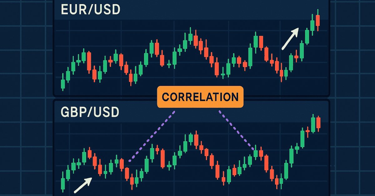
This article explains how to add currency correlation analysis to your trading toolkit. It offers practical insights and actionable strategies to enhance trading performance. Two diagrams below illustrate the market structure for EUR/USD and GBP/USD on the same dates. Both pairs were bullish on April 2 and turned bearish on April 3, demonstrating a positive correlation. Traders can use one pair to confirm reversals in the other. For example, if EUR/USD is overbought and GBP/USD is selling, that provides a clear signal of a potential reversal in EUR/USD. The Correlation Pathfinder tool is essential because it clearly shows the interrelationship between currency pairs, helping traders obtain a more accurate market picture.
GBP/USD

Fig 1. GBP/USD
EUR/USD

Fig 2. EUR/USD
System Overview
Currency correlations are expressed as a coefficient that ranges from -1 to +1. A value near +1 shows that currency pairs tend to move together, while a value near -1 signals that they move in opposite directions. A coefficient around zero indicates little or no relationship.
This understanding is vital for effective risk management. For example, buying both EUR/USD and GBP/USD during periods of strong positive correlation increases overall market exposure by effectively doubling risk. In contrast, knowing the degree of correlation enables traders to diversify portfolios and apply hedging strategies to protect against unexpected market movements, as I mentioned earlier.
The system consists of two interconnected components. First, an MQL5 Expert Advisor continuously retrieves historical price data for EUR/USD and GBP/USD. It packages this data into a JSON structure and sends it to a Python server. The second component is a Python-based analysis engine. It uses Pandas to calculate both overall and rolling correlations, and employs Matplotlib to generate a fixed-width rolling correlation graph. Furthermore, the server produces clear commentary that explains whether the currency pairs move together or diverge and outlines the implications for trading strategies.
Understand more by visualizing the following flowchart, which outlines the data flow and analysis process in the system.

Fig 3. Flow Diagram
This diagram provides a clear, visual overview of the system's workflow, tracing the process from data retrieval in MetaTrader 5 to the generation of analysis and commentary on the Python server. The nodes labeled A through H represent each step in the process, illustrating how data is collected, packaged into JSON, transmitted to the server, parsed and analyzed with Pandas, visualized with Matplotlib, and finally, accompanied by interpretative commentary before returning the analysis results.
Technical Details
The MQL5 Expert Advisor
Data Retrieval
The Expert Advisor retrieves historical price data using MetaTrader 5's built-in function, CopyRates(). This function fetches an array of price records (structured as MqlRates) that contain information such as time, open, high, low, and close prices for a given symbol and timeframe. In this EA, the user can configure the timeframe (for example, 15-minute intervals via PERIOD_M15) and the number of bars (data points) to export using the parameter BarsToExport. By allowing these values to be configurable, the EA can be tailored to various trading strategies. Whether a trader needs a short-term snapshot or a broader view of historical trends.
MqlRates rates1[];
if(CopyRates(Symbol1, TimeFrame, 0, BarsToExport, rates1) <= 0)
{
   Print("Failed to copy rates for ", Symbol1);
   return "";
}
ArraySetAsSeries(rates1, true);
Once the data is retrieved for each currency pair (such as EUR/USD and GBP/USD), the EA ensures that the data array is set as a series. This step is crucial because it arranges the array so that the most recent bar is at index 0, which aligns with how many other functions in the MQL5 environment expect data to be formatted. This preparation of historical data guarantees that the correct number of bars is retrieved and maintains the proper chronological order, which is essential for subsequent analysis.
JSON Payload Construction
After the price data is collected, the EA constructs a JSON payload that organizes the data neatly into a structured format for transmission. The BuildJSONPayload() function starts by creating a JSON object that includes the names of the two currency pairs. Then, for each currency pair, the function constructs an array of data objects. Each object in the array represents a bar of historical data and includes two key pieces of information: the time (formatted consistently using TimeToString() with parameters TIME_DATE and TIME_SECONDS) and the close price (formatted to five decimal places with DoubleToString()).
string json = "{";
json += "\"symbol1\":\"" + Symbol1 + "\",";
json += "\"symbol2\":\"" + Symbol2 + "\",";
json += "\"data1\":[";
for(int i = 0; i < ArraySize(rates1); i++)
{
   string timeStr = TimeToString(rates1[i].time, TIME_DATE | TIME_SECONDS);
   json += "{\"time\":\"" + timeStr + "\",\"close\":" + DoubleToString(rates1[i].close, 5) + "}";
   if(i < ArraySize(rates1) - 1)
      json += ",";
}
json += "],";
// The same pattern repeats for Symbol2's data array.
json += "}";
return json;
This modular approach ensures that the payload includes all necessary details for analysis on the Python server. The JSON structure makes it easier to maintain consistency and ensures that the server can parse the data without confusion. For example, by labeling the arrays as data1 and data2, the server script knows exactly which dataset corresponds to which currency pair. This clear separation is critical for merging the data later on when calculating correlation. The function iterates over each array of historical data, concatenating each record with proper JSON formatting, and then it wraps up the construction by closing the JSON object.
WebRequest Integration
Once the JSON payload is built, the EA sends the data using MetaTrader’s WebRequest() function, an essential tool for performing HTTP requests directly from the trading platform. This component handles the communication between the MQL5 Expert Advisor and the Python server that performs further analysis. Before sending the data, the EA converts the JSON string into a dynamic uchar array with the StringToCharArray() function because WebRequest() accepts the request body in this format. This conversion is necessary to ensure that the payload is transmitted correctly over the network.
string requestHeaders = "Content-Type: application/json\r\n";
uchar result[];
string responseHeaders;
int webRequestResult = WebRequest("POST", pythonUrl, requestHeaders, timeout, requestData, result, responseHeaders);
if(webRequestResult == -1)
{
   Print("Error in WebRequest. Error code = ", GetLastError());
   return;
}

string response = CharArrayToString(result);
Print("Server response: ", response);
The EA then sets up the HTTP headers, specifying that the data is in JSON format with the header "Content-Type: application/json\r\n". Configurable inputs such as the pythonUrl (the server endpoint) and timeout (how long the EA waits for a response) allow the user to fine-tune network parameters based on their environment. The WebRequest() function is used with these headers and timeout settings to send an HTTP POST request to the Python server. If the request fails, the EA prints an error code, which helps in troubleshooting connectivity issues. Otherwise, it converts the resulting uchar array response back into a string, and then prints the server’s response—this response is expected to contain useful information, such as a calculated correlation value and any commentary generated by the Python analysis engine.
The Python Analysis Server
Server Environment
The system is built on a Flask-based server that listens for POST requests. When launched, the server initializes using Flask’s default settings and sets the logging level to DEBUG. This configuration ensures that all incoming requests and processing steps are logged in detail. The server is designed to receive JSON data, process it, perform the analysis, and return results in JSON format. By using Flask, the server remains lightweight and efficient, capable of handling web requests in a headless, non-GUI environment ideal for automated trading applications.
import matplotlib
matplotlib.use("Agg")  # Use non-interactive backend to avoid GUI overhead
import matplotlib.pyplot as plt
from flask import Flask, request, jsonify
import logging

app = Flask(__name__)
logging.basicConfig(level=logging.DEBUG)

if __name__ == "__main__":
    app.run(host="127.0.0.1", port=5000)
Data Parsing and Analysis
Once the server receives a POST request, it begins by attempting to parse the incoming JSON payload. If the default parser fails, the code decodes the raw request data, trims any extraneous characters beyond the last closing curly brace, and then loads the JSON. The parsed data is then converted into two separate Pandas DataFrames, one for each currency pair. The “time” field from the payload is parsed and converted into datetime objects to facilitate accurate merging and time-series analysis. After merging the two DataFrames on the shared “Time” column, the server calculates two key correlation metrics. First, it computes the overall correlation between the closing prices of the two symbols. Second, it calculates a rolling correlation with a 50-bar window. This rolling correlation provides insights into how the correlation between the pairs changes over time, which is crucial for understanding market dynamics and spotting periods when the relationship strengthens or weakens.
import pandas as pd
import json

@app.route('/analyze', methods=['POST'])
def analyze():
    # Parse JSON payload
    data = request.get_json(silent=True)
    if not data:
        raw_data = request.data.decode('utf-8').strip()
        app.logger.debug("Raw request data: %s", raw_data)
        try:
            end_index = raw_data.rfind("}")
            trimmed_data = raw_data[:end_index+1] if end_index != -1 else raw_data
            data = json.loads(trimmed_data)
        except Exception as e:
            app.logger.error("Failed to parse JSON: %s", str(e))
            return jsonify({"error": "Invalid JSON received"}), 400

    # Convert incoming JSON arrays to DataFrames
    data1 = pd.DataFrame(data["data1"])
    data2 = pd.DataFrame(data["data2"])

    # Convert time strings to datetime objects
    data1['Time'] = pd.to_datetime(data1['time'])
    data2['Time'] = pd.to_datetime(data2['time'])

    # Merge DataFrames on 'Time'
    merged = pd.merge(data1, data2, on="Time",
                      suffixes=('_' + data["symbol1"], '_' + data["symbol2"]))

    # Calculate overall correlation between the close prices
    correlation = merged[f'close_{data["symbol1"]}'].corr(merged[f'close_{data["symbol2"]}'])

    # Calculate rolling correlation with a 50-bar window
    merged['RollingCorrelation'] = merged[f'close_{data["symbol1"]}'].rolling(window=50).corr(merged[f'close_{data["symbol2"]}'])

    # [Graph generation and commentary code follows here, see next sections]
Graph Generation and Storage
For visual representation, the server employs Matplotlib while using the “Agg” backend. This backend bypasses the need for a graphical user interface, ensuring that the plot is generated in a headless environment without triggering any GUI-related overhead. The graph is produced with a fixed figure size set to 7.5 inches wide at 100 DPI. This configuration guarantees the output image has a fixed width of 750 pixels, providing consistency across reports and making the visual data easy to interpret at a glance. Once generated, the plot displaying the rolling correlation is saved as a PNG file in the same directory as the Python script. Storing the image locally allows for easy retrieval and further sharing without including the actual graphic in the server’s JSON response.
import matplotlib.pyplot as plt

# Generate a rolling correlation plot
plt.figure(figsize=(7.5, 6), dpi=100)  # 7.5 inches * 100 dpi = 750 pixels width
plt.plot(merged['Time'], merged['RollingCorrelation'], label="Rolling Correlation (50 bars)")
plt.xlabel("Time")
plt.ylabel("Correlation")
plt.title(f"{data['symbol1']} and {data['symbol2']} Rolling Correlation")
plt.legend()
plt.grid(True)
plt.tight_layout()

# Save the graph as a PNG file in the same folder
plot_filename = "rolling_correlation.png"
plt.savefig(plot_filename)
plt.close()
Interpretative Commentary
Beyond raw numbers and graphs, the server enhances the analysis by generating interpretative commentary. This commentary is produced by a dedicated function that examines both the overall and the recent (rolling) correlation values. For example, if the overall correlation is very high (close to +1), the commentary explains that the two currency pairs generally move in tandem, which might signal the limited effectiveness of diversification when trading multiple pairs. Alternatively, if the correlation is low or becomes negative, the commentary highlights the potential for pair divergence and opportunities to hedge or adjust exposure.
def generate_commentary(corr, rolling_series):
    """Generate a commentary based on overall and recent correlation values."""
    commentary = ""
    if corr >= 0.8:
        commentary += ("The currency pairs have a very strong positive correlation, meaning "
                       "they typically move together. This may support the use of hedging strategies.\n")
    elif corr >= 0.5:
        commentary += ("The pairs display a moderately strong positive correlation with some deviations, "
                       "indicating they often move in the same direction.\n")
    elif corr >= 0.0:
        commentary += ("The overall correlation is weakly positive, suggesting occasional movement together "
                       "but limited consistency, which may offer diversification opportunities.\n")
    elif corr >= -0.5:
        commentary += ("The pairs exhibit a weak to moderate negative correlation; they tend to move in opposite "
                       "directions, which can be useful for diversification.\n")
    else:
        commentary += ("The pairs have a strong negative correlation, implying they generally move in opposite "
                       "directions, a factor exploitable in hedging strategies.\n")

    if not rolling_series.empty:
        recent_trend = rolling_series.iloc[-1]
        commentary += f"Recently, the rolling correlation is at {recent_trend:.2f}. "
        if recent_trend > 0.8:
            commentary += ("This high correlation suggests near mirror-like movement. "
                           "Relative strength approaches may need reconsideration for diversification.")
        elif recent_trend < 0.3:
            commentary += ("A significant drop in correlation indicates potential decoupling. "
                           "This may signal opportunities in pair divergence trades.")
        else:
            commentary += ("The correlation remains moderate, meaning the pairs show some synchronization but also "
                           "retain independent movement.")
    return commentary
The commentary also offers insights into recent trends in correlation, providing traders with practical guidance on what these statistical signals could mean for their risk management and strategy. By combining quantitative analysis with qualitative insights, the system helps traders better understand market behavior and make more informed decisions.
Outcomes
Before we delve into the outcomes, it is necessary to explain how to initiate the Python server. First, download and install Python from python.org and set up a virtual environment by running python -m venv venv and activating it. Next, install the required packages by executing pip install Flask pandas matplotlib. Create a Python script (for example, server.py) containing your Flask server code and the necessary endpoints. Finally, navigate to the script’s directory and run the server with python server.py. Please refer to one of my previous articles on external flow for further details.
Below is a presentation of test outcomes conducted on the EUR/USD and GBP/USD pairs. For best results, ensure you test the system on the same pairs specified in your EA. Initially, the command prompt logs indicate that the system was successfully initialized, and they clearly display the data relayed from MetaTrader 5 by the MQL5 EA to the Python server—this includes the open, close, and time values for the period from April 2 to April 9. The log entry, "POST /analyze HTTP/1.1" 200, confirms a successful connection and that the Python server executed the required processing as expected.
DEBUG:plotter:Raw request data: {"symbol1":"EURUSD","symbol2":"GBPUSD","data1":[{"time":"2025.04.09 07:00:00"
,"close":1.10766},{"time":"2025.04.09 06:45:00","close":1.10735},{"time":"2025.04.09 06:30:00","close":1.10602}
,{"time":"2025.04.09 06:15:00","close":1.10538},{"time":"2025.04.09 06:00:00","close":1.10486},
{"time":"2025.04.09 05:45:00","close":1.10615},{"time":"2025.04.09 05:30:00","close":1.10454},
{"time":"2025.04.09 05:15:00","close":1.10402},{"time":"2025.04.09 05:00:00","close":1.10447},
{"time":"2025.04.09 04:45:00","close":1.10685},{"time":"2025.04.09 04:30:00","close":1.10582},
{"time":"2025.04.09 04:15:00","close":1.10617},{"time":"2025.04.09 04:00:00","close":1.10384},
{"time":"2025.04.09 03:45:00","close":1.10196},{"time":"2025.04.09 03:30:00","close":1.10184},
{"time":"2025.04.09 03:15:00","close":1.10339},{"time":"2025.04.09 03:00:00","close":1.10219},
{"time":"2025.04.09 02:45:00","close":1.10197},{"time":"2025.04.09 02:30:00","close":1.10130},
{"time":"2025.04.09 02:15:00","close":1.10233},{"time":"2025.04.09 02:00:00","close":1.10233},
{"time":"2025.04.09 01:45:00","close":1.10200},{"time":"2025.04.09 01:30:00","close":1.10289},
{"time":"2025.04.09 01:15:00","close":1.10382},{"time":"2025.04.09 01:00:00","close":1.10186},
{"time":"2025.04.09 00:45:00","close":1.10148},{"time":"2025.04.09 00:30:00","close":1.09985},
{"time":"2025.04.09 00:15:00","close":1.09894},{"time":"2025.04.09 00:00:00","close":1.09747},
{"time":"2025.04.08 23:45:00","close":1.09776},{"time":"2025.04.08 23:30:00","close":1.09789},
{"time":"2025.04.08 23:15:00","close":1.09793},{"time":"2025.04.08 23:00:00","close":1.09740},
{"time":"2025.04.08 22:45:00","close":1.09681},{"time":"2025.04.08 22:30:00","close":1.09718},
{"time":"2025.04.08 22:15:00","close":1.09669},{"time":"2025.04.08 22:00:00","close":1.09673},
{"time":"2025.04.08 21:45:00","close":1.09586},{"time":"2025.04.08 21:30:00","close":1.09565},
{"time":"2025.04.08 21:15:00","close":1.09507},{"time":"2025.04.08 21:00:00","close":1.09493},
{"time":"2025.04.08 20:45:00","close":1.09529},{"time":"2025.04.08 20:30:00","close":1.09442},
{"time":"2025.04.08 20:15:00","close":1.09417},{"time":"2025.04.08 20:00:00","close":1.09533},
{"time":"2025.04.08 19:45:00","close":1.09541},{"time":"2025.04.08 19:30:00","close":1.09587},
{"time":"2025.04.08 19:15:00","close":1.09684},{"time":"2025.04.08 19:00:00","close":1.09724},
{"time":"2025.04.08 18:45:00","close":1.09521},{"time":"2025.04.08 18:30:00","close":1.09551},
{"time":"2025.04.08 18:15:00","close":1.09561},{"time":"2025.04.08 18:00:00","close":1.09474},
{"time":"2025.04.08 17:45:00","close":1.09337},{"time":"2025.04.08 17:30:00","close":1.09334},
{"time":"2025.04.08 17:15:00","close":1.09421},{"time":"2025.04.08 17:00:00","close":1.09429},
{"time":"2025.04.08 16:45:00","close":1.09296},{"time":"2025.04.08 16:30:00","close":1.09210},
{"time":"2025.04.08 16:15:00","close":1.09123},{"time":"2025.04.08 16:00:00","close":1.09073},
{"time":"2025.04.08 15:45:00","close":1.09116},{"time":"2025.04.08 15:30:00","close":1.09083},
{"time":"2025.04.08 15:15:00","close":1.09119},{"time":"2025.04.08 15:00:00","close":1.08986},
{"time":"2025.04.08 14:45:00","close":1.09102},{"time":"2025.04.08 14:30:00","close":1.08954},
{"time":"2025.04.08 14:15:00","close":1.09051},{"time":"2025.04.08 14:00:00","close":1.09213},
{"time":"2025.04.08 13:45:00","close":1.09357},{"time":"2025.04.08 13:30:00","close":1.09300},
{"time":"2025.04.08 13:15:00","close":1.09548},{"time":"2025.04.08 13:00:00","close":1.09452},
{"time":"2025.04.08 12:45:00","close":1.09485},{"time":"2025.04.08 12:30:00","close":1.09585},
{"time":"2025.04.08 12:15:00","close":1.09477},{"time":"2025.04.08 12:00:00","close":1.09512},
{"time":"2025.04.08 11:45:00","close":1.09342},{"time":"2025.04.08 11:30:00","close":1.09311},
{"time":"2025.04.07 09:45:00","close":1.09627},{"time":"2025.04.07 09:30:00","close":1.09545},
{"time":"2025.04.07 09:15:00","close":1.09597},{"time":"2025.04.07 09:00:00","close":1.09729},
{"time":"2025.04.07 08:45:00","close":1.09918},{"time":"2025.04.07 08:30:00","close":1.09866},
{"time":"2025.04.07 08:15:00","close":1.09705},{"time":"2025.04.07 08:00:00","close":1.10051},
{"time":"2025.04.07 07:45:00","close":1.10006},{"time":"2025.04.07 07:30:00","close":1.10232},
{"time":"2025.04.07 07:15:00","close":1.10273},{"time":"2025.04.07 07:00:00","close":1.10397},
{"time":"2025.04.07 06:45:00","close":1.10029},{"time":"2025.04.07 06:30:00","close":1.10083},
{"time":"2025.04.07 06:15:00","close":1.10012},{"time":"2025.04.07 06:00:00","close":1.10084},
{"time":"2025.04.07 05:45:00","close":1.10183},{"time":"2025.04.07 05:30:00","close":1.09905},
{"time":"2025.04.07 05:15:00","close":1.09941},{"time":"2025.04.07 05:00:00","close":1.09826},
{"time":"2025.04.07 04:45:00","close":1.09848},{"time":"2025.04.07 04:30:00","close":1.09830},
{"time":"2025.04.07 04:15:00","close":1.09739},{"time":"2025.04.07 04:00:00","close":1.09608},
{"time":"2025.04.07 03:45:00","close":1.09503},{"time":"2025.04.07 03:30:00","close":1.09456},
{"time":"2025.04.07 03:15:00","close":1.09373},{"time":"2025.04.07 03:00:00","close":1.09343},
{"time":"2025.04.07 02:45:00","close":1.09353},{"time":"2025.04.07 02:30:00","close":1.09248},
{"time":"2025.04.07 02:15:00","close":1.09360},{"time":"2025.04.07 02:00:00","close":1.09550},
{"time":"2025.04.07 01:45:00","close":1.09673},{"time":"2025.04.07 01:30:00","close":1.09740},
{"time":"2025.04.07 01:15:00","close":1.09688},{"time":"2025.04.07 01:00:00","close":1.09649},
{"time":"2025.04.07 00:45:00","close":1.09667},{"time":"2025.04.07 00:30:00","close":1.09526},
{"time":"2025.04.07 00:15:00","close":1.09555},{"time":"2025.04.07 00:00:00","close":1.09517},
{"time":"2025.04.06 23:45:00","close":1.09825},{"time":"2025.04.06 23:30:00","close":1.09981},
{"time":"2025.04.06 23:15:00","close":1.09872},{"time":"2025.04.06 23:00:00","close":1.09981},
{"time":"2025.04.06 22:45:00","close":1.09822},{"time":"2025.04.06 22:30:00","close":1.09803},
{"time":"2025.04.06 22:15:00","close":1.09826},{"time":"2025.04.06 22:00:00","close":1.09529},
{"time":"2025.04.06 21:45:00","close":1.09147},{"time":"2025.04.06 21:30:00","close":1.09046},
{"time":"2025.04.06 21:15:00","close":1.08910},{"time":"2025.04.06 21:00:00","close":1.08818},
{"time":"2025.04.04 20:45:00","close":1.09623},{"time":"2025.04.04 20:30:00","close":1.09435},
{"time":"2025.04.04 20:15:00","close":1.09339},{"time":"2025.04.04 20:00:00","close":1.09502},
{"time":"2025.04.04 19:45:00","close":1.09436},{"time":"2025.04.04 19:30:00","close":1.09631},
{"time":"2025.04.04 19:15:00","close":1.09425},{"time":"2025.04.04 19:00:00","close":1.09358},
{"time":"2025.04.04 18:45:00","close":1.09447},{"time":"2025.04.04 18:30:00","close":1.09611},
{"time":"2025.04.04 18:15:00","close":1.09604},{"time":"2025.04.04 18:00:00","close":1.09531},
{"time":"2025.04.04 17:45:00","close":1.09472},{"time":"2025.04.04 17:30:00","close":1.09408},
{"time":"2025.04.04 17:15:00","close":1.09311},{"time":"2025.04.04 17:00:00","close":1.09407},
{"time":"2025.04.04 16:45:00","close":1.09714},{"time":"2025.04.04 16:30:00","close":1.09690},
{"time":"2025.04.04 16:15:00","close":1.09845},{"time":"2025.04.04 16:00:00","close":1.09892},
{"time":"2025.04.04 15:45:00","close":1.10139},{"time":"2025.04.04 15:30:00","close":1.09998},
{"time":"2025.04.04 15:15:00","close":1.09837},{"time":"2025.04.04 15:00:00","close":1.09970},
{"time":"2025.04.04 14:45:00","close":1.09862},{"time":"2025.04.04 14:30:00","close":1.09706},
{"time":"2025.04.04 14:15:00","close":1.09991},{"time":"2025.04.04 14:00:00","close":1.10068},
{"time":"2025.04.04 13:45:00","close":1.10057},{"time":"2025.04.04 13:30:00","close":1.10252},
{"time":"2025.04.04 13:15:00","close":1.10288},{"time":"2025.04.04 13:00:00","close":1.10358},
{"time":"2025.04.04 12:45:00","close":1.10200},{"time":"2025.04.04 12:30:00","close":1.10289},
{"time":"2025.04.04 12:15:00","close":1.10794},{"time":"2025.04.04 12:00:00","close":1.10443},
{"time":"2025.04.04 11:45:00","close":1.10601},{"time":"2025.04.04 11:30:00","close":1.10697},
{"time":"2025.04.04 11:15:00","close":1.10502},{"time":"2025.04.04 11:00:00","close":1.10517},
{"time":"2025.04.04 10:45:00","close":1.10305},{"time":"2025.04.04 10:30:00","close":1.10340},
{"time":"2025.04.04 10:15:00","close":1.10447},{"time":"2025.04.04 10:00:00","close":1.09869},
{"time":"2025.04.04 09:45:00","close":1.09844},{"time":"2025.04.04 09:30:00","close":1.09757},
{"time":"2025.04.04 09:15:00","close":1.09820},{"time":"2025.04.04 09:00:00","close":1.09786},
{"time":"2025.04.04 08:45:00","close":1.09962},{"time":"2025.04.04 08:30:00","close":1.10002},
{"time":"2025.04.04 08:15:00","close":1.10062},{"time":"2025.04.04 08:00:00","close":1.10034},
{"time":"2025.04.04 07:45:00","close":1.10042},{"time":"2025.04.04 07:30:00","close":1.10223},
{"time":"2025.04.04 07:15:00","close":1.10490},{"time":"2025.04.04 07:00:00","close":1.10641},
{"time":"2025.04.04 06:45:00","close":1.10506},{"time":"2025.04.04 06:30:00","close":1.10638},
{"time":"2025.04.04 06:15:00","close":1.10649},{"time":"2025.04.04 06:00:00","close":1.10747},
{"time":"2025.04.04 05:45:00","close":1.10843},{"time":"2025.04.04 05:30:00","close":1.10809},
{"time":"2025.04.04 05:15:00","close":1.11057},{"time":"2025.04.04 05:00:00","close":1.10984},
{"time":"2025.04.04 04:45:00","close":1.10874},{"time":"2025.04.04 04:30:00","close":1.10896},
{"time":"2025.04.04 04:15:00","close":1.10906},{"time":"2025.04.04 04:00:00","close":1.10876},
{"time":"2025.04.04 03:45:00","close":1.10937},{"time":"2025.04.04 03:30:00","close":1.10918},
{"time":"2025.04.04 03:15:00","close":1.10766},{"time":"2025.04.04 03:00:00","close":1.10695},
{"time":"2025.04.04 02:45:00","close":1.10632},{"time":"2025.04.04 02:30:00","close":1.10668},
{"time":"2025.04.04 02:15:00","close":1.10625},{"time":"2025.04.04 02:00:00","close":1.10773},
{"time":"2025.04.04 01:45:00","close":1.10677},{"time":"2025.04.04 01:30:00","close":1.10625},
{"time":"2025.04.04 01:15:00","close":1.10610},{"time":"2025.04.04 01:00:00","close":1.10589},
{"time":"2025.04.04 00:45:00","close":1.10606},{"time":"2025.04.04 00:30:00","close":1.10603},
{"time":"2025.04.04 00:15:00","close":1.10403},{"time":"2025.04.04 00:00:00","close":1.10432},
{"time":"2025.04.03 23:45:00","close":1.10452},{"time":"2025.04.03 23:30:00","close":1.10467},
{"time":"2025.04.03 23:15:00","close":1.10446},{"time":"2025.04.03 23:00:00","close":1.10524},
{"time":"2025.04.03 22:45:00","close":1.10642},{"time":"2025.04.03 22:30:00","close":1.10631},
{"time":"2025.04.03 22:15:00","close":1.10582},{"time":"2025.04.03 22:00:00","close":1.10577},
{"time":"2025.04.03 21:45:00","close":1.10515},{"time":"2025.04.03 21:30:00","close":1.10497},
{"time":"2025.04.03 21:15:00","close":1.10505},{"time":"2025.04.03 21:00:00","close":1.10488},
{"time":"2025.04.03 20:45:00","close":1.10514},{"time":"2025.04.03 20:30:00","close":1.10448},
{"time":"2025.04.03 20:15:00","close":1.10312},{"time":"2025.04.03 20:00:00","close":1.10253},
{"time":"2025.04.03 19:45:00","close":1.10275},{"time":"2025.04.03 19:30:00","close":1.10164},
{"time":"2025.04.03 19:15:00","close":1.10192},{"time":"2025.04.03 19:00:00","close":1.10320},
{"time":"2025.04.03 18:45:00","close":1.10373},{"time":"2025.04.03 18:30:00","close":1.10362},
{"time":"2025.04.03 18:15:00","close":1.10322},{"time":"2025.04.03 18:00:00","close":1.10236},
{"time":"2025.04.03 17:45:00","close":1.10245},{"time":"2025.04.03 17:30:00","close":1.10222},
{"time":"2025.04.03 17:15:00","close":1.10273},{"time":"2025.04.03 17:00:00","close":1.10267},
{"time":"2025.04.03 16:45:00","close":1.10386},{"time":"2025.04.03 16:30:00","close":1.10404},
{"time":"2025.04.03 16:15:00","close":1.10367},{"time":"2025.04.03 16:00:00","close":1.10491},
{"time":"2025.04.03 15:45:00","close":1.10506},{"time":"2025.04.03 15:30:00","close":1.10452},
{"time":"2025.04.03 15:15:00","close":1.10613},{"time":"2025.04.03 15:00:00","close":1.10922},
{"time":"2025.04.03 14:45:00","close":1.11182},{"time":"2025.04.03 14:30:00","close":1.11197},
{"time":"2025.04.03 14:15:00","close":1.10950},{"time":"2025.04.03 14:00:00","close":1.10981},
{"time":"2025.04.03 13:45:00","close":1.10784},{"time":"2025.04.03 13:30:00","close":1.10911},
{"time":"2025.04.03 13:15:00","close":1.10943},{"time":"2025.04.03 13:00:00","close":1.11064},
{"time":"2025.04.03 12:45:00","close":1.10816},{"time":"2025.04.03 12:30:00","close":1.10910},
{"time":"2025.04.03 12:15:00","close":1.10858},{"time":"2025.04.03 12:00:00","close":1.10867},
{"time":"2025.04.03 11:45:00","close":1.10876},{"time":"2025.04.03 11:30:00","close":1.10839},
{"time":"2025.04.03 11:15:00","close":1.10570},{"time":"2025.04.03 11:00:00","close":1.10596},
{"time":"2025.04.03 10:45:00","close":1.10521},{"time":"2025.04.03 10:30:00","close":1.10696},
{"time":"2025.04.03 10:15:00","close":1.10859},{"time":"2025.04.03 10:00:00","close":1.11052},
{"time":"2025.04.03 09:45:00","close":1.10305},{"time":"2025.04.03 09:30:00","close":1.10280},
{"time":"2025.04.03 09:15:00","close":1.10336},{"time":"2025.04.03 09:00:00","close":1.10304},
{"time":"2025.04.03 08:45:00","close":1.10093},{"time":"2025.04.03 08:30:00","close":1.10092},
{"time":"2025.04.03 08:15:00","close":1.09885},{"time":"2025.04.03 08:00:00","close":1.09803},
{"time":"2025.04.03 07:45:00","close":1.09707},{"time":"2025.04.03 07:30:00","close":1.09658},
{"time":"2025.04.03 07:15:00","close":1.09497},{"time":"2025.04.03 07:00:00","close":1.09733},
{"time":"2025.04.03 06:45:00","close":1.09896},{"time":"2025.04.03 06:30:00","close":1.09775},
{"time":"2025.04.03 06:15:00","close":1.09488},{"time":"2025.04.03 06:00:00","close":1.09457},
{"time":"2025.04.03 05:45:00","close":1.09444},{"time":"2025.04.03 05:30:00","close":1.09515},
{"time":"2025.04.03 05:15:00","close":1.09431},{"time":"2025.04.03 05:00:00","close":1.09171},
{"time":"2025.04.03 04:45:00","close":1.09069},{"time":"2025.04.03 04:30:00","close":1.09104},
{"time":"2025.04.03 04:15:00","close":1.09109},{"time":"2025.04.03 04:00:00","close":1.09110},
{"time":"2025.04.03 03:45:00","close":1.09148},{"time":"2025.04.03 03:30:00","close":1.09118},
{"time":"2025.04.03 03:15:00","close":1.09196},{"time":"2025.04.03 03:00:00","close":1.09115},
{"time":"2025.04.03 02:45:00","close":1.09122},{"time":"2025.04.03 02:30:00","close":1.09207},
{"time":"2025.04.03 02:15:00","close":1.09220},{"time":"2025.04.03 02:00:00","close":1.09134},
{"time":"2025.04.03 01:45:00","close":1.09132},{"time":"2025.04.03 01:30:00","close":1.09137},
{"time":"2025.04.03 01:15:00","close":1.09078},{"time":"2025.04.03 01:00:00","close":1.08970},
{"time":"2025.04.03 00:45:00","close":1.08906},{"time":"2025.04.03 00:30:00","close":1.08995},
{"time":"2025.04.03 00:15:00","close":1.08831},{"time":"2025.04.03 00:00:00","close":1.08905},
{"time":"2025.04.02 23:45:00","close":1.09044},{"time":"2025.04.02 23:30:00","close":1.09068},
{"time":"2025.04.02 23:15:00","close":1.08874},{"time":"2025.04.02 23:00:00","close":1.08552},
{"time":"2025.04.02 22:45:00","close":1.08389},{"time":"2025.04.02 22:30:00","close":1.08277},
{"time":"2025.04.02 22:15:00","close":1.08221},{"time":"2025.04.02 22:00:00","close":1.08161},
{"time":"2025.04.02 21:45:00","close":1.08274},{"time":"2025.04.02 21:30:00","close":1.08286},
{"time":"2025.04.02 21:15:00","close":1.08156},{"time":"2025.04.02 21:00:00","close":1.08350},
{"time":"2025.04.02 20:45:00","close":1.08507},{"time":"2025.04.02 20:30:00","close":1.08184},
INFO:werkzeug:127.0.0.1 - - [09/Apr/2025 09:04:18] "POST /analyze HTTP/1.1" 200 -
Below are logs from the MetaTrader 5 Experts tab, which include the Python server's commentary on the correlation analysis. The logs detail data received from previous days up to the current day, showing how the two currency pairs, EUR/USD and GBP/USD, have moved in relation to one another. The commentary interprets the correlation plot, explaining that, over the recorded period, the pairs generally maintain a strong positive correlation.
2025.04.09 00:57:33.296 Correlation Pathfinder (GBPUSD,M15)     Server response:
{"commentary":"The overall correlation is weakly positive, suggesting occasional movement together but
limited consistency, which may offer diversification opportunities.\nRecently, the rolling correlation is at
0.82. This high correlation suggests near mirror-like movement. Relative strength approaches may need
reconsideration for diversification.","correlation":0.3697032305325312,"message":"Plot saved as rolling_
correlation.png"}
This indicates that they tend to move in tandem, though slight deviations have occurred at times. These deviations may suggest temporary market divergence, highlighting potential opportunities for portfolio diversification or hedging. Overall, the logs confirm successful data transmission and accurate processing, offering insights that can help refine trading strategies based on the evolving relationship between the currency pairs.
2025.04.09 00:
57 :33.296 Correlation Pathfinder (EURUSD,M15)     Server response:
{"commentary":"The overall correlation is weakly positive, suggesting occasional movement together but
limited consistency, which may offer diversification opportunities.\nRecently, the rolling correlation is at
 0.83. This high correlation suggests near mirror-like movement. Relative strength approaches may need
reconsideration for diversification.","correlation":0.33874205977082567,"message":"Plot saved as
rolling_correlation.png"}
Below is our correlation plot analysis. From April 2 to April 9 the rolling correlation between EUR/USD and GBP/USD stayed high near 0.8 to 1.0, showing that the pairs generally moved together. There were moments when the correlation dropped sharply to about 0.3, which indicates a brief divergence likely due to short-lived market events or currency-specific news. The correlation quickly recovered back toward 1.0, confirming that the underlying market forces realign these pairs. Traders can use these occasional dips as signals for divergence opportunities and then monitor until normal correlation levels return.

Fig 4. Rolling Correlation
Conclusion
This diagram provides a clear, visual overview of the system's workflow, tracing the process from data retrieval in MetaTrader 5 to the generation of analysis and commentary on the Python server. The nodes labeled A through H represent each step in the process, illustrating how data is collected, packaged into JSON, transmitted to the server, parsed and analyzed with Pandas, visualized with Matplotlib, and finally, accompanied by interpretative commentary before returning the analysis results.
| Date | Tool Name | Description | Version | Updates | Notes |
|---|---|---|---|---|---|
| 01/10/24 | Chart Projector | Script to overlay the previous day's price action with a ghost effect. | 1.0 | Initial Release | Tool number 1 |
| 18/11/24 | Analytical Comment | It provides previous day's information in a tabular format, as well as anticipates the future direction of the market. | 1.0 | Initial Release | Tool number 2 |
| 27/11/24 | Analytics Master | Regular Update of market metrics after every two hours | 1.01 | Second Release | Tool number 3 |
| 02/12/24 | Analytics Forecaster | Regular Update of market metrics after every two hours with telegram integration | 1.1 | Third Edition | Tool number 4 |
| 09/12/24 | Volatility Navigator | The EA analyzes market conditions using the Bollinger Bands, RSI and ATR indicators | 1.0 | Initial Release | Tool Number 5 |
| 19/12/24 | Mean Reversion Signal Reaper | Analyzes market using mean reversion strategy and provides signal | 1.0 | Initial Release | Tool number 6 |
| 9/01/25 | Signal Pulse | Multiple timeframe analyzer | 1.0 | Initial Release | Tool number 7 |
| 17/01/25 | Metrics Board | Panel with button for analysis | 1.0 | Initial Release | Tool number 8 |
| 21/01/25 | External Flow | Analytics through external libraries | 1.0 | Initial Release | Tool number 9 |
| 27/01/25 | VWAP | Volume Weighted Average Price | 1.3 | Initial Release | Tool number 10 |
| 02/02/25 | Heikin Ashi | Trend Smoothening and reversal signal identification | 1.0 | Initial Release | Tool number 11 |
| 04/02/25 | FibVWAP | Signal generation through python analysis | 1.0 | Initial Release | Tool number 12 |
| 14/02/25 | RSI DIVERGENCE | Price action versus RSI divergences | 1.0 | Initial Release | Tool number 13 |
| 17/02/25 | Parabolic Stop and Reverse (PSAR) | Automating PSAR strategy | 1.0 | Initial Release | Tool number 14 |
| 20/02/25 | Quarters Drawer Script | Drawing quarters levels on chart | 1.0 | Initial Release | Tool number 15 |
| 27/02/25 | Intrusion Detector | Detect and alert when price reaches quarters levels | 1.0 | Initial Release | Tool number 16 |
| 27/02/25 | TrendLoom Tool | Multi timeframe analytics panel | 1.0 | Initial Release | Tool number 17 |
| 11/03/25 | Quarters Board | Panel with buttons to activate or disable quarters levels | 1.0 | Initial Release | Tool number 18 |
| 26/03/25 | ZigZag Analyzer | Drawing trendlines using ZigZag Indicator | 1.0 | Initial Release | Tool number 19 |
| 10/04/25 | Correlation Pathfinder | Plotting currency correlations using Python libraries. | 1.0 | Initial Release | Tool number 20 |
- Free trading apps
- Over 8,000 signals for copying
- Economic news for exploring financial markets
You agree to website policy and terms of use