Reimagining Classic Strategies (Part 14): High Probability Setups

In our previous discussions, we have analyzed how trading moving average cross-overs can be reimagined by fixing the periods of the 2 moving average indicators in question. We demonstrated that by doing so, we can effectively exercise a reasonable level of control over the amount of lag in our trading strategy. We proceeded to observe that, by applying one moving average on the opening price level and the other on the closing price level, we obtained a much more sensitive form of the legacy moving average cross-over strategy.  Our new framework, yields some guarantees we could not obtain from the traditional strategy. Readers who have not yet read that previous discussion we had, can find the article readily available, here.

Today, we are further exploring whether there is any merit in trying to yield more productivity from our reimagined version of moving average cross-over. By carefully modelling the relationship between our moving average cross-over strategy, and the EURUSD market, we can hopefully learn what the difference is, between the market conditions in which our strategy excels and the market conditions which prove too challenging for our strategy. Our goal, is to then build a trading strategy that learns to stop trading when it detects unfavorable market conditions.

Overview of The Trading Strategy

It is widely accepted, by most members of our community, that traders should actively seek to trade high probability setups. However, there are few formal definitions of what exactly constitutes a high probability trading setup. How do we empirically measure the probability associated with any particular trading setup? Depending on who you ask, you will get different definitions of how you can identify such opportunities and take advantage of them responsibly.

This article seeks to address these issues by proposing an algorithmic framework that allows us to depart from old definitions, and lean towards numerical definitions that are evidence based, so that our trading strategies may be able to identify and trade them profitably, all by themselves in a consistent manner. 

We desire to model the relationship between our particular trading strategy and any Symbol we have chosen to trade. We can achieve this by first fetching market data that fully describes the market, and all the parameters that make up our trading strategy, all from the MetaTrader 5 terminal.
Afterward, we will fit a statistical model to classify if the strategy is going to produce signals that are profitable, or if the signal being generated by our strategy is most likely going to be unprofitable. 

The probability estimated by our model, becomes the probabilities we associate with that particular signal. Hence, we can now start talking about "high probability setups" in a more scientific and empirical way, that is reasoned from evidence and relevent market data.

This framework essentially allows us to write trading strategies that are "goal aware", and explicitly instructed to only take actions they expect to be favorable. We are beginning to formalize the necessary components needed to write algorithmic trading strategies, that try to estimate, the the most probable consequences of their actions. This can be correctly conceptualised as reinforcement learning ideologies, being approached in a supervised fashion.

Getting Started In MQL5

Our task today is centered on learning the relationship between our trading strategy and the Symbol we wish to trade. To achieve this goal, we will fetch the growth in the 4 primary price feeds (Open, High, Low and Close) as well as the changes in our two moving average indicators. 

Note that, for labelling the data, we will also need to have the original real values of the two indicators and the closing price. All in all, we will write out our data into a CSV file with 10 columns, and then proceed to learning the relationship our strategy has with this particular Symbol and at every step of the way, we will contrast this result against the performance of an identical model, trying to predict the market price directly.

This will inform us which target is easier to learn, and the beauty of our approach, is the simple fact that regardless of which target is easier to forecast, they both inform us where price is going.

/+-------------------------------------------------------------------+
//|                                                      ProjectName |
//|                                      Copyright 2020, CompanyName |
//|                                       http://www.companyname.net |
//+------------------------------------------------------------------+
#property copyright "Copyright 2024, MetaQuotes Ltd."
#property link      "https://www.mql5.com"
#property version   "1.00"
#property script_show_inputs

//--- Define our moving average indicator
#define MA_PERIOD 3                 //--- Moving Average Period
#define MA_TYPE   MODE_SMA          //--- Type of moving average we have
#define  HORIZON 10

//--- Our handlers for our indicators
int ma_handle,ma_o_handle;

//--- Data structures to store the readings from our indicators
double ma_reading[],ma_o_reading[];

//--- File name
string file_name = Symbol() + " Reward Modelling.csv";

//--- Amount of data requested
input int size = 3000;

//+------------------------------------------------------------------+
//| Our script execution                                             |
//+------------------------------------------------------------------+
void OnStart()
  {
   int fetch = size + (HORIZON * 2);
//---Setup our technical indicators
   ma_handle = iMA(_Symbol,PERIOD_CURRENT,MA_PERIOD,0,MA_TYPE,PRICE_CLOSE);
   ma_o_handle = iMA(_Symbol,PERIOD_CURRENT,MA_PERIOD,0,MA_TYPE,PRICE_OPEN);

//---Set the values as series
   CopyBuffer(ma_handle,0,0,fetch,ma_reading);
   ArraySetAsSeries(ma_reading,true);
   CopyBuffer(ma_o_handle,0,0,fetch,ma_o_reading);
   ArraySetAsSeries(ma_o_reading,true);

//---Write to file
   int file_handle=FileOpen(file_name,FILE_WRITE|FILE_ANSI|FILE_CSV,",");

   for(int i=size;i>=1;i--)
     {
      if(i == size)
        {
         FileWrite(file_handle,"Time","True Close","True MA C","True MA O","Open","High","Low","Close","MA Close 2","MA Open 2");
        }

      else
        {
         FileWrite(file_handle,
                   iTime(_Symbol,PERIOD_CURRENT,i),
                   iClose(_Symbol,PERIOD_CURRENT,i),
                   ma_reading[i],
                   ma_o_reading[i],
                   iOpen(_Symbol,PERIOD_CURRENT,i)   - iOpen(_Symbol,PERIOD_CURRENT,(i + HORIZON)),
                   iHigh(_Symbol,PERIOD_CURRENT,i)   - iHigh(_Symbol,PERIOD_CURRENT,(i + HORIZON)),
                   iLow(_Symbol,PERIOD_CURRENT,i)    - iLow(_Symbol,PERIOD_CURRENT,(i + HORIZON)),
                   iClose(_Symbol,PERIOD_CURRENT,i)  - iClose(_Symbol,PERIOD_CURRENT,(i + HORIZON)),
                   ma_reading[i] - ma_reading[(i + HORIZON)],
                   ma_o_reading[i] - ma_o_reading[(i + HORIZON)]
                  );
        }
     }
//--- Close the file
   FileClose(file_handle);
  }
//+------------------------------------------------------------------+

Analyzing The Data

To get started, let's read in our market data into a Jupyter Notebook so we can perform our numerical analysis of the strategy's performance.

import pandas as pd

Define how far into the future we would like to forecast our Profits or Losses.

HORIZON = 10

Read in the data and add the columns we need. The first column, 'Target', is the traditional market return, in this case it is the 10 day EURUSD market return. The column 'Class' is either 1 for bullish days, otherwise its 0.  Thirdly, the 'Action' column denotes what action our trading strategy would've been triggered to make, 1 corresponds to buying and -1 to selling. The 'Reward' column is calculated as the element wise product of the 'Target' column and the 'Action' column, this multiplication will only produce positive rewards if our strategy:

• Chose action -1 and the classical target was less than 0 (this means our strategy sold and future price levels depreciated)
• Chose action 1 and the classical target exceeded than 0 (this means our strategy bought and future price levels appreciated)

Any other combination of actions and targets would produce negative rewards because our trading strategy acted inappropriately. If our classifier can learn to predict whether our reward will be positive, we would have effectively found a very reliable tool to keep us out of unfavorable market conditions, and help us to place our trades when they are most likely to pay off. The last column, 'Trade Signal' is set to 0 and only set to 1 if our reward is positive. Initially, all 5 columns will be set to 0.

data = pd.read_csv("..\EURUSD Reward Modelling.csv")

data['Target'] = 0
data['Class']  = 0
data['Action'] = 0
data['Reward'] = 0
data['Trade Signal'] = 0

Now, we fill in our classical target, the 10-day change in the EURUSD closing price.

data['Target'] = data['True Close'].shift(-HORIZON) - data['True Close']
data.dropna(inplace=True)

We need to label the classes, so we can distinguish bullish and bearish days quickly in our plots.

data.loc[data['Target'] > 0,'Class'] = 1

Let us now fill in which actions our strategy would've taken.

data.loc[data['True MA C'] > data['True MA O'],'Action'] = 1
data.loc[data['True MA C'] < data['True MA O'],'Action'] = -1

And the profit or loss our strategy would've made for taking those actions.

data['Reward'] = data['Target'] * data['Action']

Now, let us fill in the trading signal which tells us if we should act or wait.

data.loc[((data['Target'] < 0) & (data['Action'] == -1)),'Trade Signal'] = 1
data.loc[((data['Target'] > 0) & (data['Action'] == 1)),'Trade Signal'] = 1

We can take a look at the data. We can quickly see that it is challenging to separate the market action well. The orange dots represent trade signals that we should've taken, while the blue, represents signals we should've ignored. The fact that the orange and blue dots can be seen on top of each other in this scatter plot, mathematically informs the reader that profitable and unprofitable trade signals can form under almost identical conditions. Our statistical models may be able to spot the similarities and differences that we as humans aren't sensitive enough to recognize, or would require considerable labor to do so.

import numpy as np
import seaborn as sns
import matplotlib.pyplot as plt

sns.scatterplot(data=data,x='MA Close 2',y='MA Open 2',hue='Trade Signal')
plt.title('Analyzing How Well Moving Average Cross Overs Separate The Market')
plt.grid()

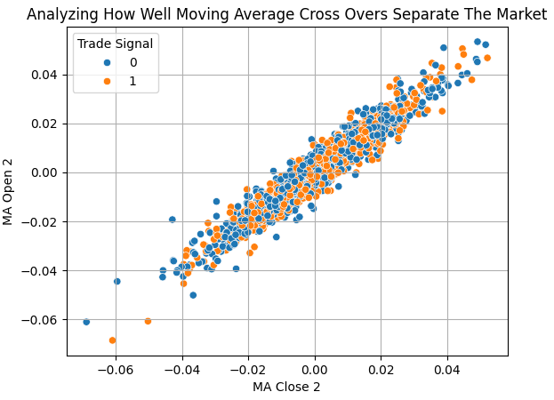
Fig 1: Our moving average cross-overs appear to have challenges separating price action

Let us quickly estimate if our new target, is easier to forecast than the traditional target. 

from sklearn.linear_model import RidgeClassifier
from sklearn.model_selection import TimeSeriesSplit,cross_val_score

Linear models are particularly useful for getting reliable and inexpensive approximations. Let's create a time-series split object so we can cross-validate a linear classifier.

tscv = TimeSeriesSplit(n_splits=5,gap=HORIZON)
model = RidgeClassifier()
scores = []

Cross-validate the model, first on the legacy target, then lastly on our new target which is trying to estimate the profit/loss generated by our strategy. Since we are performing a classification task, be sure to set the scoring method to 'accuracy'.

scores.append(np.mean(np.abs(cross_val_score(model,data.iloc[:,4:-5],data.loc[:,'Class'],cv=tscv,scoring='accuracy'))))
scores.append(np.mean(np.abs(cross_val_score(model,data.iloc[:,4:-5],data.loc[:,'Trade Signal'],cv=tscv,scoring='accuracy'))))

Creating a bar-plot of the results quickly reveals that the model forecasting the strategy's profit/loss is outperforming the model attempting to forecast the market directly. The model trying to forecast the model directly fell below the 50% threshold, while our new target is helping us cross the 50% benchmark, though only marginally above the barrier in all honesty.

sns.barplot(scores,color='black')
plt.axhline(np.max(scores),linestyle=':',color='red')
plt.title('Forcasting Market Returns vs Forecasting Strategy Reward')
plt.ylabel('Percentage Accuracy Levels %')
plt.xlabel('0: Market Return Forecast | 1: Strategy Profit/Loss Forecast')

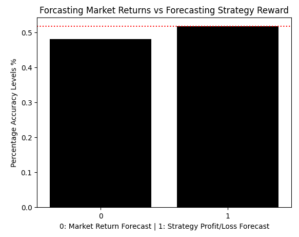
Fig 2: Our linear models are suggesting to us that we may be better off forecasting the profit or loss generated by our strategy

We can calculate the exact percentage increase in performance we have gained, and it appears that we benefit a 7.6% increase in accuracy by forecasting the relationship between the strategy and the market over forecasting the market directly.

scores = (((scores / scores[0]) - 1) * 100)

scores[1]

7.595993322203687

Drop all the data that overlaps with our back-test period so that our back test represents a material simulation of real market conditions.

#Drop all the data that overlaps with your backtest period
data = data.iloc[:-((365 * 4) + (30 * 5) + 17),:]
data

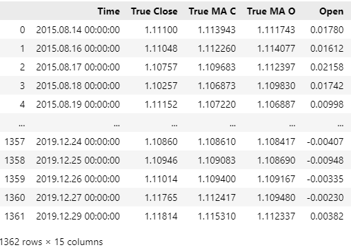
Fig 3: Ensure that the dates you have on your data frame do not overlap the dates we will back-test over

The linear model gave us confidence that forecasting profit/loss generated by the strategy may be better for us than forecasting price directly. However, we will use a more flexible learner in our trading back-tests to ensure that the model is picking up as much useful information as possible.

from sklearn.ensemble import GradientBoostingRegressor

model = GradientBoostingRegressor()

Label the inputs and the target.

X = ['Open','High','Low','Close','MA Close 2','MA Open 2']
y = 'Trade Signal'

Fit the model.

model.fit(data.loc[:,X],data.loc[:,y])

Prepare to export the model to ONNX.

import onnx
from skl2onnx import convert_sklearn
from skl2onnx.common.data_types import FloatTensorType

Define the model's input size.

initial_types = [("float input",FloatTensorType([1,6]))]

Save the model.

onnx_proto = convert_sklearn(model,initial_types=initial_types,target_opset=12)
onnx.save(onnx_proto,"EURUSD Reward Model.onnx")

Getting Started in MQL5

We are now ready to commence the development of our trading application. We shall build two versions of the strategy to assess the effectiveness of our changes to the training procedure for our statistical model. Both versions of the trading algorithm will be back tested under identical conditions. Let us familiarize ourselves with these particular conditions so that we do not have to duplicate the same information unnecessarily. 

The first important setting is the symbol, as we have already discussed, we are trading the EURUSD pair in this example. We will trade the Symbol on the daily time-frame over a period of 5 years, from 1 January 2020 until 1 April 2025. This will give us a large period to examine the merit of our application. The reader should recall that in Fig 3, we effectively erased any market data we had beyond 29 December 2019.

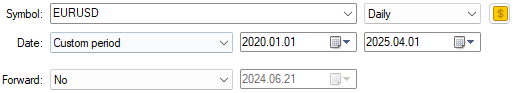
Fig 4: The dates needed for our back test across both versions of our trading strategy

Lastly, the conditions which we will model the market will be set to mimic the unpredictable nature of real trading. Therefore, we have chosen to use our delay to be set to Random delay, and have every tick based on real ticks, to obtain a realistic rendition of the market. 

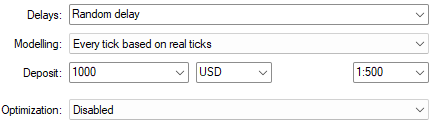
Fig 5: The settings we will use to mimic the market conditions are materially important

Let us now start building an application we can back-test to assess the merit of the changes we have proposed to our training procedure. We will start off by measuring the performance of our strategy without using the new modelling approach we have formulated to identify high probability setups. In essence, the first version of our trading strategy is just applying the discretionary trading strategy of trading the moving average cross-overs when they happen. This will give us a benchmark that we will use to compare our proposed reward modelling strategy against. To get us started, we will begin by importing the trade library.

//+------------------------------------------------------------------+
//|                                             Reward Modelling.mq5 |
//|                                               Gamuchirai Ndawana |
//|                    https://www.mql5.com/en/users/gamuchiraindawa |
//+------------------------------------------------------------------+
#property copyright "Gamuchirai Ndawana"
#property link      "https://www.mql5.com/en/users/gamuchiraindawa"
#property version   "1.00"

//+------------------------------------------------------------------+
//| Libraries we need                                                |
//+------------------------------------------------------------------+
#include <Trade\Trade.mqh>
CTrade Trade;

Define useful system constants, these constants match the other constants we used in both the MQL5 Script and the Python script.

//+------------------------------------------------------------------+
//| System constants                                                 |
//+------------------------------------------------------------------+
#define MA_PERIOD 3                //--- Moving Average Period
#define MA_TYPE   MODE_SMA         //--- Type of moving average we have
#define HORIZON 10                 //--- How far into the future we should forecast

Set up our global variables and technical indicators.

//+------------------------------------------------------------------+
//| Global variables                                                 |
//+------------------------------------------------------------------+
int fetch = HORIZON + 1;

//+------------------------------------------------------------------+
//| Technical indicators                                             |
//+------------------------------------------------------------------+
int ma_handle,ma_o_handle;
double ma_reading[],ma_o_reading[];
int position_timer;

Each event handler has been paired with a corresponding method that will be called when the handler is triggered. This design style will keep you codebase easier to maintain and extend in the future if you think of new ideas. Directly writing your code in the event handler itself will require the developer to carefully parse through numerous lines of code before making any changes to be sure nothing will break whereas with our design pattern, the developer needs only to stack a call to his desired function above the ones we have provided, if he wishes to extend the functionality of the application.

//+------------------------------------------------------------------+
//| Expert initialization function                                   |
//+------------------------------------------------------------------+
int OnInit()
  {
//---
   if(!setup())
      return(INIT_FAILED);
//---
   return(INIT_SUCCEEDED);
  }
  
//+------------------------------------------------------------------+
//| Expert deinitialization function                                 |
//+------------------------------------------------------------------+
void OnDeinit(const int reason)
  {
//---
   release();
  }
  
//+------------------------------------------------------------------+
//| Expert tick function                                             |
//+------------------------------------------------------------------+
void OnTick()
  {
//---
   update();
  }
//+------------------------------------------------------------------+

Now we shall consider each method in turn. The first function we will set up is the function responsible for loading our technical indicators and resetting our position timer. The position timer is needed to ensure that we hold each trade for as long as our horizon system constant is set.

//+------------------------------------------------------------------+
//| Setup the system                                                 |
//+------------------------------------------------------------------+
bool setup(void)
  {
//---Setup our technical indicators
   ma_handle = iMA(_Symbol,PERIOD_CURRENT,MA_PERIOD,0,MA_TYPE,PRICE_CLOSE);
   ma_o_handle = iMA(_Symbol,PERIOD_CURRENT,MA_PERIOD,0,MA_TYPE,PRICE_OPEN);
   position_timer = 0;

   return(true);
  }

The release method simply frees up the technical indicators we aren't using, it is good practice in MQL5 to clean up after yourself.

//+------------------------------------------------------------------+
//| Release system variables we are no longer using                  |
//+------------------------------------------------------------------+
void release(void)
  {
   IndicatorRelease(ma_handle);
   IndicatorRelease(ma_o_handle);
   return;
  }

The update method will fetch current price levels and copy them into our indicator buffers. Additionally, it will also keep track of how long our current position has been open to close it on time.

//+------------------------------------------------------------------+
//| Update system parameters                                         |
//+------------------------------------------------------------------+
void update(void)
  {
   //--- Time stamps
   static datetime time_stamp;
   datetime current_time = iTime(Symbol(),PERIOD_D1,0);

   //--- We are on a new day
   if(time_stamp != current_time)
     {
      time_stamp = current_time;
      if(PositionsTotal() == 0)
        {
         //--- Copy indicator values
         CopyBuffer(ma_handle,0,0,fetch,ma_reading);
         CopyBuffer(ma_o_handle,0,0,fetch,ma_o_reading);
         //---Set the values as series
         ArraySetAsSeries(ma_reading,true);
         ArraySetAsSeries(ma_o_reading,true);
         find_setup();
         position_timer = 0;
        }

      //--- Forecasts are only valid for HORIZON days
      if(PositionsTotal() > 0)
        {
         position_timer += 1;
        }

      //--- Otherwise close the position
      if(position_timer == HORIZON)
         Trade.PositionClose(Symbol());
     }
     return;
  }

And lastly, the find setup function. Our setups are identified whenever we have moving average cross-overs. If the open crosses above the close, that registers as a short signal. Otherwise, we have a long signal.

//+------------------------------------------------------------------+
//| Find a trading oppurtunity                                       |
//+------------------------------------------------------------------+
void find_setup(void)
  {
         double bid = SymbolInfoDouble(Symbol(),SYMBOL_BID) , ask = SymbolInfoDouble(Symbol(),SYMBOL_ASK);
         double vol = SymbolInfoDouble(Symbol(),SYMBOL_VOLUME_MIN);

         vector ma_o,ma_c;

         ma_o.CopyIndicatorBuffer(ma_o_handle,0,0,1);
         ma_c.CopyIndicatorBuffer(ma_handle,0,0,1);

         if(ma_o[0] > ma_c[0])
           {
            Trade.Sell(vol,Symbol(),ask,0,0,"");
           }

         if(ma_o[0] < ma_c[0])
           {
            Trade.Buy(vol,Symbol(),bid,0,0,"");
           }
     return;
  }    

Do not forget to undefine the system constants we defined earlier.

//+------------------------------------------------------------------+
//| Undefine system constatns                                        |
//+------------------------------------------------------------------+
#undef HORIZON
#undef MA_PERIOD
#undef MA_TYPE

We have already covered the settings we will use for our back test just prior. Our goal is to observe how effective our strategy is, devoid of the statistical modelling techniques we developed. Simply load the expert advisor, and then start the back test using the settings we discussed in Fig 4 and 5.

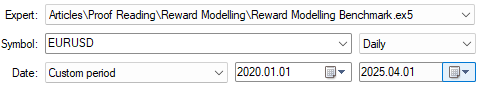
Fig 6: Establishing a benchmark

Our discretionary version of the trading strategy was profitable, although it appears to be marginally profitable. The difference between the average profit and loss is only $0.9 and only 51% of all the trades it places are profitable, this isn't very encouraging. Our Sharpe ratio is 0.62 and could possibly improve if we revamped our system.

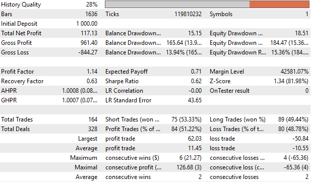
Fig 7: A detailed analysis of the performance of our discretionary trading strategy

Now when we analyze the balance and equity curve produced by this version of the trading strategy, we can immediately see obvious flaws. The strategy is unstable and volatile. In fact, 4 years into the back test, by February 2024, the strategy almost returned to its opening balance at the beginning of the back test. It struggled to break out of an unprofitable series of trades from late 2020 running 4 years into 2024. This is not attractive for us as algorithmic traders. 

Fig 8: Visualizing the profit and loss curve generated by our discretionary version of the trading strategy

Improving The Performance of Our Expert Advisor

Now let us improve our trading strategy by giving our application the ability to mimic the human thought process of considering the consequences of your actions before committing yourself. 

We will start off by first importing our ONNX model into the application as a resource from our system file directory. 

//+------------------------------------------------------------------+
//| System resources                                                 |
//+------------------------------------------------------------------+
#resource "\\Files\\EURUSD Reward Model.onnx" as uchar onnx_proto[];

A few additional global variables will be required to make use of our model. Primarily we need variables to represent the model handler, and the amount of data we should fetch.

//+------------------------------------------------------------------+
//| Global variables                                                 |
//+------------------------------------------------------------------+
long onnx_model;
int fetch = HORIZON + 1;

Moving on, we now need to set up the ONNX model in the setup function. In the code example below, we have deliberately omitted code segments that haven't changed across both versions of the application. We simply create the ONNX model from its buffer, validate the model and then specify its input and output size accordingly. If any step along the way were to fail, we will abort the initialization procedure completely.

//+------------------------------------------------------------------+
//| Setup the system                                                 |
//+------------------------------------------------------------------+
bool setup(void)
  {
//---Omitted code that hasn't changed

//--- Setup the ONNX model
   onnx_model = OnnxCreateFromBuffer(onnx_proto,ONNX_DEFAULT);

//--- Validate the ONNX model
   if(onnx_model == INVALID_HANDLE)
     {
      Comment("Failed to create ONNX model");
      return(false);
     }

//--- Register the ONNX model I/O parameters
   ulong input_shape[] = {1,6};
   ulong output_shape[] = {1,1};

   if(!OnnxSetInputShape(onnx_model,0,input_shape))
     {
      Comment("Failed to set input shape");
      return(false);
     }

   if(!OnnxSetOutputShape(onnx_model,0,output_shape))
     {
      Comment("Failed to set output shape");
      return(false);
     }

   return(true);
  }

Additionally, when the application is released, we will need to release system resources we aren't using anymore

//+------------------------------------------------------------------+
//| Release system variables we are no longer using                  |
//+------------------------------------------------------------------+
void release(void)
  {
//--- Omitted code segments that haven't changed
   OnnxRelease(onnx_model);
   return;
  }

We will instruct the application to first obtain a forecast from our trading model before deciding if it should place a trade. If our model's forecast is above 0.5, that means our algorithm is expecting the signal generated by our strategy to be profitable and gives us permission to trade. If that is not the case, then we will wait for the unfavorable market conditions to run their course.

//+------------------------------------------------------------------+
//| Find a trading oppurtunity                                       |
//+------------------------------------------------------------------+
void find_setup(void)
  {
//--- Skipped parts of the code base that haven't changed

//--- Prepare the model's inputs
   vectorf model_input(6);
   model_input[0] = (float)(iOpen(_Symbol,PERIOD_CURRENT,0)   - iOpen(_Symbol,PERIOD_CURRENT,(HORIZON)));
   model_input[1] = (float)(iHigh(_Symbol,PERIOD_CURRENT,0)   - iHigh(_Symbol,PERIOD_CURRENT,(HORIZON)));
   model_input[2] = (float)(iLow(_Symbol,PERIOD_CURRENT,0)    - iLow(_Symbol,PERIOD_CURRENT,(HORIZON)));
   model_input[3] = (float)(iClose(_Symbol,PERIOD_CURRENT,0)  - iClose(_Symbol,PERIOD_CURRENT,(HORIZON)));
   model_input[4] = (float)(ma_reading[0] - ma_reading[(HORIZON)]);
   model_input[5] = (float)(ma_o_reading[0] - ma_o_reading[(HORIZON)]);

//--- Prepare the model's output
   vectorf model_output(1);

//--- We failed to run the model
   if(!OnnxRun(onnx_model,ONNX_DATA_TYPE_FLOAT,model_input,model_output))
      Comment("Failed to obtain a forecast");

//--- Everything went fine
   else
     {
      Comment("Forecast: ",model_output[0]);

      //--- Our model forecasts that our strategy is likely to be profitable
      if(model_output[0] > 0.5)
        {
         if(ma_o[0] > ma_c[0])
           {
            Trade.Sell(vol,Symbol(),ask,0,0,"");
           }

         if(ma_o[0] < ma_c[0])
           {
            Trade.Buy(vol,Symbol(),bid,0,0,"");
           }
        }
     }
   return;
  }

Run the application in a back test using the settings specified in Fig 4 and 5 to make a fair comparison between the two strategies.

Fig 9: Running our second back test using our revised version of the trading strategy that models profit and losses

Our Sharpe Ratio increased from 0.62 in the discretionary benchmark applying the same strategy, to 1.07 in our current iteration, this represents an increase of 72%. Our total net profit appreciated by 38% from $117.13, to $162.75 when following the new algorithmically defined "high probability setup" strategy. The proportion of losing trades fell by 17% from 48.78% to 40.48%. And lastly, the total trades placed by the strategy fell from 164 to 126, meaning that our new system made 38% more profit with just 76% of the total number of trades used by the old system, effectively meaning we are more effective than we were before because we are making greater returns while taking on less risk.

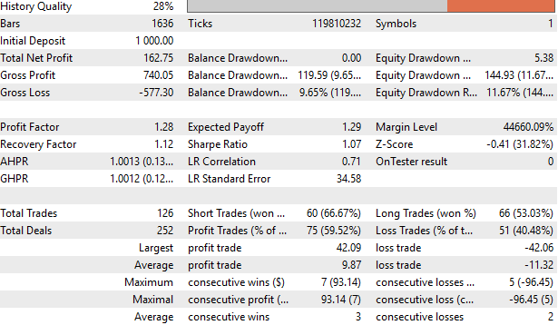
Fig 10: A detailed summary of the performance of our new trading strategy

I have provided the reader with the balance and equity curve of the revised version of our trading strategy, and I placed the curve produced by the original version of the strategy underneath so that the reader can make comparisons between them without having to scroll back and forth. We can clearly see that before the first back tested year was over, the original version of our trading strategy, was almost reverting to the break even point, while our new strategy handled that period well. 

It's interesting to note that both strategies struggled to perform during the May – December 2022 period. This may be a sign of particularly unstable market periods that will need more effort to be effectively addressed.

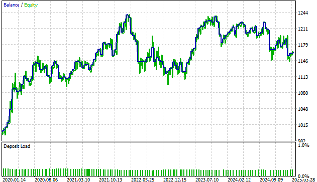
Fig 11: The profit and loss curve produced by our new trading strategy that has the ability to consider the consequences of its actions

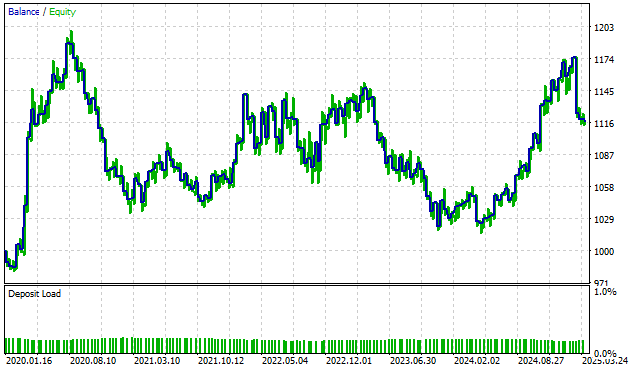
Fig 12: The equity curve produced by the original version of our trading strategy has been copied for easier comparison against the new results we have produced

Conclusion

After reading this article, the reader has learned a novel way to approach the task of algorithmically trading using supervised statistical models. The reader is now furnished with the knowledge needed to model the relationships that exist between their private trading strategies and the markets they trade. This yields the reader a competitive advantage over casual market participants attempting to forecast the market directly, which we have shown is not always the best option available to the reader. 

File Name	File Description
Reward Modelling Benchmark.mq5	This is the traditional version of our trading strategy that makes no attempt to consider the consequences of its actions. It equally weights all trading opportunities and assumes that each trade must be profitable.
Reward Modelling.mq5	This is the refined version of our trading strategy that explicitly tries to estimate the consequences of its actions before placing any trades.
EURUSD Reward Model.onnx	Our ONNX statistical model that estimates the probability that the signal generated by our strategy will be profitable.
Reward Modelling.ipynb	The Jupyter Notebook we used to analyze our historical market data and fit our statistical model.