Neural Networks in Trading: Transformer for the Point Cloud (Pointformer)

Introduction
Object detection in point clouds is important for many real-world applications. Compared to images, point clouds offer detailed geometric information and can effectively capture scene structure. However, their irregular nature presents significant challenges for efficient feature learning.
Transformer-based architectures have achieved remarkable success in natural language processing. They are effective in learning context-dependent representations and model long-range dependencies within input sequences. The Transformer, along with its Self-Attention mechanism, not only satisfies the requirement for permutation invariance but also demonstrates high expressive power. Nevertheless, directly applying Transformers to point clouds is computationally prohibitive, as the cost increases quadratically with input size.
To address this issue, the authors of the method Pointformer, introduced in the paper "3D Object Detection with Pointformer", proposed an approach that uses the strengths of Transformer models when dealing with set-structured data. Pointformer adopts a U-Net structure composed of multi-scale Pointformer blocks. Each Pointformer block consists of Transformer-based modules designed to be both highly expressive and well-suited for object detection tasks.
In their architectural solution, the method authors use three Transformer modules:
- Local Transformer (LT) models interactions between points within a local region. It learns context-aware features at the object level.
- Local-Global Transformer (LGT) facilitates the integration of local and global features with higher resolution.
- Global Transformer (GT) captures context-dependent representations at the scene level.
As a result, Pointformer effectively models both local and global dependencies, significantly improving feature learning performance in complex scenes with multiple cluttered objects.
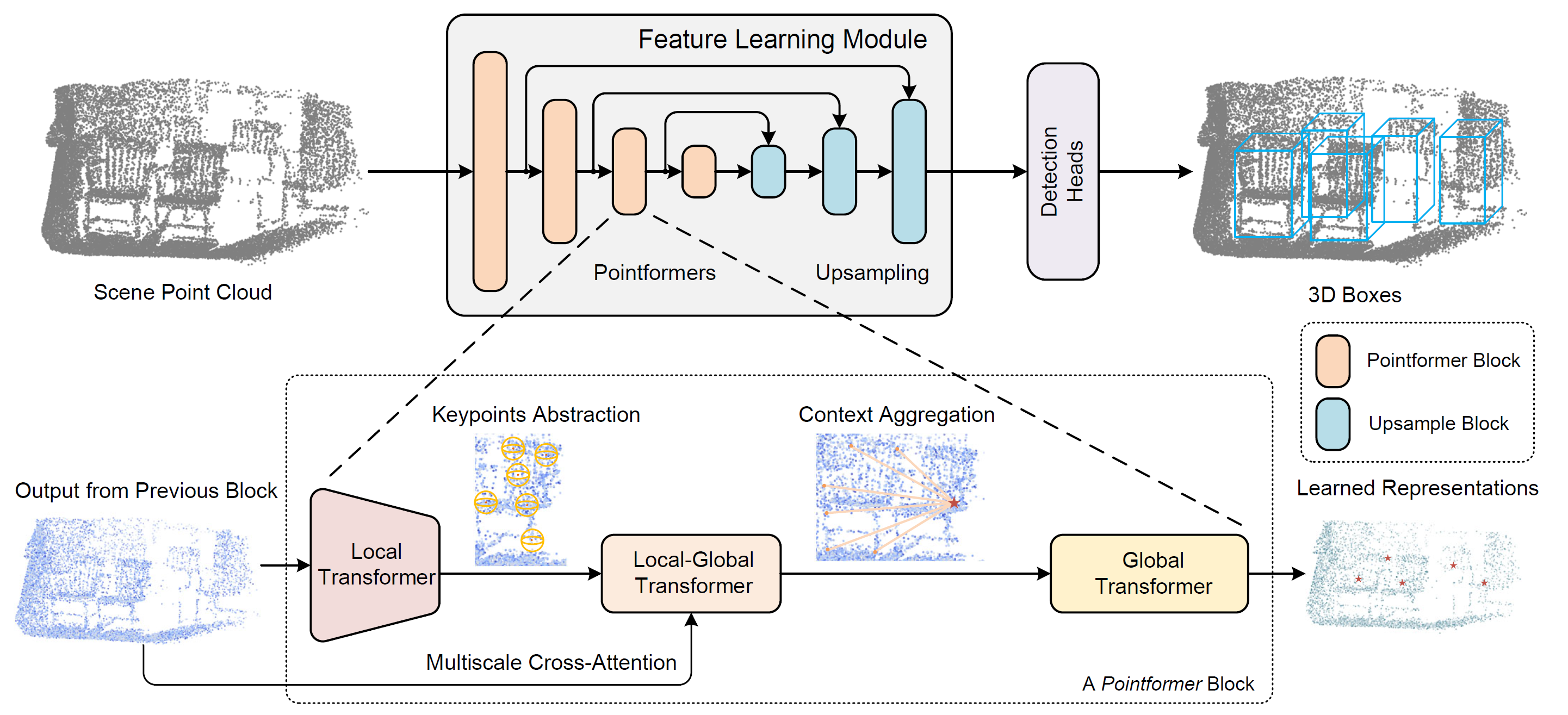
1. The Pointformer Algorithm
When processing point clouds, it is essential to consider their irregular, unordered nature and varying sizes. The authors of Pointformer developed Transformer-based modules specifically designed for point set operations. These modules not only enhance the expressiveness of local feature extraction but also incorporate global contextual information into point representations.
The Pointformer block consists of three modules: Local Transformer (LT), Local-Global Transformer (LGT) and Global Transformer (GT). Each block begins with the LT, which receives high-resolution input from the previous layer and extracts features for a new, lower-resolution point set. Next, the LGT module applies a multi-scale cross-attention mechanism to integrate features from both resolutions. Finally, the GT module captures scene-level context-aware representations. For upsampling, the authors adopt the feature propagation module from PointNet++.
To construct a hierarchical representation of the point cloud scene, Pointformer employs a high-level methodology that builds feature learning blocks at different resolutions. Initially, Farthest Point Sampling (FPS) is used to select a subset of points to serve as centroids. For each centroid, a local neighborhood is defined by selecting surrounding points within a specified radius. These local groups are then organized into sequences and fed into a Transformer layer. A shared Transformer block is applied to all local regions. As more Transformer layers are stacked within a Pointformer block, the expressiveness of the module increases, leading to improved feature representations.
The method also takes into account feature correlations among neighboring points. Adjacent points may sometimes provide more informative context than the centroid itself. By enabling information exchange among all points within a local region, the model treats each point equally, resulting in more effective local feature extraction.
Farthest Point Sampling (FPS) is widely used in point cloud systems due to its ability to produce nearly uniform sample distributions while preserving the overall shape of the input. This ensures broad coverage of the original point cloud with a limited number of centroids. However, FPS has two major drawbacks:
- It is sensitive to outliers, which can lead to high instability, especially when dealing with real-world point clouds.
- FPS selects points that are a strict subset of the original point cloud, which can hinder accurate geometry reconstruction, particularly in cases of partial object occlusion or sparsely sampled objects.
Since most points lie on the surfaces of objects, the second issue is especially critical. Sampling-based proposal generation can result in a natural disconnect between proposal quality and actual object presence.
To overcome these limitations, the authors of Pointformer introduce a coordinate refinement module based on Self-Attention maps. This module first extracts the Self-Attention maps from the final Transformer layer for each attention head. Then, the attention maps are averaged. After that, the refined centroid coordinates are calculated by applying attention-weighted averaging across all points within the local region. This process adaptively shifts centroid coordinates closer to the actual centers of objects.
Global context, including inter-object boundary correlations and scene-level information, is also valuable for object detection tasks. Pointformer uses the ability of Transformer modules to model long-range, non-local dependencies. In particular, the Global Transformer module is designed to transmit information across the entire point cloud. All points are collected into one group and serve as the initial data for the GT module.
The use of a Transformer at the scene level enables the capture of context-sensitive representations and facilitates information exchange between different objects. These global representations are especially beneficial for detecting objects that are represented by only a few points.
The Local-Global Transformer is also a key module for combining local and global functions extracted by LT and GT modules. LGT uses a multi-scale cross-attention mechanism to establish relationships between low-resolution centroids and high-resolution points. Formally, it uses a Transformer cross-attention mechanism. LT results serve as Queries, while higher-resolution GT outputs serve as Keys and Values.
Positional encoding is a fundamental component of Transformer models, providing a means to incorporate position information into the input sequence. When adapting Transformers to point cloud data, positional encoding becomes even more important, as point coordinates themselves are highly informative and critical for capturing local geometric structures.
Author's visualization of the Pointformer method is presented below.
2. Implementation in MQL5
After reviewing the theoretical aspects of the Pointformer method, we now move on to the practical part of the article, where we implement our interpretation of the proposed approaches using MQL5.
Upon closer examination of the proposed approaches, we can notice some similarities with the PointNet++ method. Both algorithms use the Farthest Point Sampling mechanism to form centroids. The basic operations of both methods are based on grouping points around centroids. That is why i decided to use the CNeuronPointNet2OCL object as a parent for constructing the new CNeuronPointFormer class. Its structure is presented below.
class CNeuronPointFormer   :  public CNeuronPointNet2OCL
  {
protected:
   CNeuronMLMHSparseAttention    caLocalAttention[2];
   CNeuronMLCrossAttentionMLKV   caLocalGlobalAttention[2];
   CNeuronMLMHAttentionMLKV      caGlobalAttention[2];
   CNeuronLearnabledPE           caLocalPE[2];
   CNeuronLearnabledPE           caGlobalPE[2];
   CNeuronBaseOCL                cConcatenate;
   CNeuronConvOCL                cScale;
   //---
   CBufferFloat                 *cbTemp;
   //---
   virtual bool      feedForward(CNeuronBaseOCL *NeuronOCL) override ;
   //---
   virtual bool      calcInputGradients(CNeuronBaseOCL *NeuronOCL) override;
   virtual bool      updateInputWeights(CNeuronBaseOCL *NeuronOCL) override;

public:
                     CNeuronPointFormer(void) {};
                    ~CNeuronPointFormer(void) { delete cbTemp; }
   //---
   virtual bool      Init(uint numOutputs, uint myIndex, COpenCLMy *open_cl,
                          uint window, uint units_count, uint output, bool use_tnets,
                          ENUM_OPTIMIZATION optimization_type, uint batch) override;
   //---
   virtual int       Type(void) override   const   {  return defNeuronPointFormer; }
   //---
   virtual bool      Save(int const file_handle) override;
   virtual bool      Load(int const file_handle) override;
   //---
   virtual bool      WeightsUpdate(CNeuronBaseOCL *source, float tau) override;
   virtual void      SetOpenCL(COpenCLMy *obj) override;

  };
In CNeuronPointNet2OCL, we used 2 scale levels to extract local features. In the new class, we keep a similar level of scaling, but we take the quality of feature extraction to a new level by using the proposed attention modules. This improvement is reflected in the internal arrays of neural layers, whose purpose will become clear during the implementation of the methods in our new CNeuronPointFormer class.
Among the internal components, there is only one dynamically allocated buffer, which we will properly deallocate in the class destructor. The class constructor will remain empty. The initialization of all internal objects will be performed in the Init method, whose parameters are copied from the parent class.
bool CNeuronPointFormer::Init(uint numOutputs, uint myIndex, COpenCLMy *open_cl,

                              uint window, uint units_count, uint output, bool use_tnets,
                              ENUM_OPTIMIZATION optimization_type, uint batch)
  {
   if(!CNeuronPointNet2OCL::Init(numOutputs, myIndex, open_cl, window, units_count, output,
                                                      use_tnets, optimization_type, batch))
      return false;
In the body of the method, we begin by calling the corresponding method from the parent class, which controls the received parameters and initializes the inherited objects.
In the parent class, we create two internal layers of local subsampling. Each of these layers outputs a 64-dimensional feature vector for every point in the input point cloud.
Following each local subsampling layer, we will insert attention modules as proposed by the authors of the Pointformer method. The architecture of the attention modules for both layers will be identical, so we will initialize the objects within a loop.
   for(int i = 0; i < 2; i++)
     {
      if(!caLocalAttention[i].Init(0, i*5, OpenCL, 64, 16, 4, units_count, 2, optimization, iBatch))
         return false;
First, we initialize the local attention module, which is implemented using the CNeuronMLMHSparseAttention block.
It should be noted that our approach slightly diverges from the original Pointformer algorithm. However, we believe it retains the core logic. In the Pointformer method, the local attention module enriches each point in a local region with shared contextual features, thereby focusing attention on the object as a whole. Clearly, points belonging to the same object exhibit strong interdependencies. By using sparse attention, we are not restricted to a fixed local region but can instead emphasize points with high relational significance. This is similar to identifying support and resistance levels in technical analysis, where price repeatedly interacts with specific thresholds across different historical segments.
Next, we initialize the local-global attention module, which integrates fine-grained context from the original data into the features of local objects.
      if(!caLocalGlobalAttention[i].Init(0, i*5+1, OpenCL, 64, 16, 4, 64, 2, units_count,
                                                   units_count, 2, 2, optimization, iBatch))
         return false;
The global attention block is used to identify context-dependent representations at the scene level.
      if(!caGlobalAttention[i].Init(0, i*5+2, OpenCL, 64, 16, 4, 2, units_count, 2, 2, optimization, iBatch))
         return false;
And of course we will add internal layers of trainable positional coding. Here we use separate positional encoding for local and global representation.
      if(!caLocalPE[i].Init(0, i*5+3, OpenCL, 64*units_count, optimization, iBatch))
         return false;
      if(!caGlobalPE[i].Init(0, i*5+4, OpenCL, 64*units_count, optimization, iBatch))
         return false;
     }
It is important to mention that we do not implement the centroid coordinate refinement block proposed by the Pointformer authors. First, in our implementation of PointNet++, we designated each point in the cloud as a centroid of its local region. Thus, altering point coordinates could distort the overall scene. Second, part of the refinement function is inherently handled by the trainable positional encoding layers.
A brief note on feature extraction scaling. The initialized modules themselves do not explicitly indicate different feature extraction scales. However, there are two points. In the parent class, we used varying radii for local subsampling. Here, we will introduce different levels of sparsity in the local attention modules.
   caLocalAttention[0].Sparse(0.1f);
   caLocalAttention[1].Sparse(0.3f);
We concatenate the results of two global attention levels into a single tensor.
   if(!cConcatenate.Init(0, 10, OpenCL, 128 * units_count, optimization, iBatch))
      return false;
Then we reduce its dimensionality down to the level of the original data of the global point cloud descriptor extraction block, which was initialized in the parent class method.
   if(!cScale.Init(0, 11, OpenCL, 128, 128, 64, units_count, 1, optimization, iBatch))
      return false;
At the end of the initialization method, we add the creation of a buffer for storing intermediate data.
   if(!!cbTemp)
      delete cbTemp;
   cbTemp = new CBufferFloat();
   if(!cbTemp ||
      !cbTemp.BufferInit(caGlobalAttention[0].Neurons(), 0) ||
      !cbTemp.BufferCreate(OpenCL))
      return false;
//---
   return true;
  }
After that, we return the logical result of the operations to the calling program and complete the method.
The next stage of development involves implementing the feed-forward pass algorithm within the feedForward method. Unlike the initialization method, here we cannot fully rely on the corresponding method from the parent class. In this new method, we must integrate operations involving both inherited and newly introduced components.
As before, the forward pass method receives a pointer to the input data object as one of its parameters. In the method body, we immediately store this pointer in a local variable.
bool CNeuronPointFormer::feedForward(CNeuronBaseOCL *NeuronOCL)
  {
//--- LocalNet
   CNeuronBaseOCL *inputs = NeuronOCL;
Typically, we avoid storing incoming pointers in local variables unless necessary. However, in this case, we are implementing an algorithm that involves sequential processing by two nested feature extraction blocks operating at different scales. Within this context, working with a local variable simplifies the logic, as it allows us to reassign the pointer to different objects during iteration.
Next, we proceed to create the above-mentioned loop.
   for(int i = 0; i < 2; i++)
     {
      if(!cTNetG || i > 0)
        {
         if(!caLocalPointNet[i].FeedForward(inputs))
            return false;
        }
Inside the loop, we begin with local subsampling operations, using the objects that were declared and initialized in the parent class.
It is important to recall that the parent class algorithm includes an option to project input data into a canonical space. This operation is only applied before the first layer of local subsampling. Therefore, at the beginning of the loop, we check whether this projection is required. If not, we proceed directly with the local subsampling step.
If projection is required, we first generate the projection matrix.
      else
        {
         if(!cTurnedG)
            return false;
         if(!cTNetG.FeedForward(inputs))
            return false;
Then we implement the projection of the original data.
         int window = (int)MathSqrt(cTNetG.Neurons());
         if(IsStopped() ||
            !MatMul(NeuronOCL.getOutput(), cTNetG.getOutput(), cTurnedG.getOutput(),
                                           NeuronOCL.Neurons() / window, window, window))
            return false;
Only after this we perform subsampling of local data.
         if(!caLocalPointNet[i].FeedForward(cTurnedG.AsObject()))
            return false;
        }
The output from the local subsampling layer is passed directly into the local attention module.
      //--- Local Attention
      if(!caLocalAttention[i].FeedForward(caLocalPointNet[i].AsObject()))
         return false;
It is important to note that we pass the data into the local attention module without positional encoding. I would like to remind you that the Self-Attention mechanism is inherently invariant to the order of the input elements. Therefore, within the local attention block, we identify elements with strong mutual influence, regardless of their spatial coordinates.
At first glance, the phrase "local attention without coordinate dependence" may sound counterintuitive. After all, local attention seems to imply some spatial or positional restriction. But let's look at it from a different perspective. Consider a price chart. We can split the information into two categories: coordinates and features. In this analogy, time serves as the coordinate, while the price level represents the feature. If we remove the coordinates (time), we are left with a point cloud in feature space. The regions where the price level occurs more frequently will naturally have a higher density of points. These points may be far apart in time. Yet often such areas correspond to support and resistance levels. In this sense, our local attention module operates within a local feature space.
After this step, we apply positional encoding both to the output of the local attention module and to the output of the local subsampling layer.
      //--- Position Encoder
      if(!caLocalPE[i].FeedForward(caLocalAttention[i].AsObject()))
         return false;
      if(!caGlobalPE[i].FeedForward(caLocalPointNet[i].AsObject()))
         return false;
And in the next step, in the local-global attention module, we enrich the local attention data with information from the global context, taking into account the coordinates of the objects.
      //--- Local to Global Attention
      if(!caLocalGlobalAttention[i].FeedForward(caLocalPE[i].AsObject(), caGlobalPE[i].getOutput()))
         return false;
And the operations of our loop are completed by the global attention module, in which the information of objects is enriched with the general context of the scene.
      //--- Global Attention
      if(!caGlobalAttention[i].FeedForward(caLocalGlobalAttention[i].AsObject()))
         return false;
      inputs = caGlobalAttention[i].AsObject();
     }
Before moving on to the next iteration of the loop, we make sure to change the pointer to the source data object in the local variable.
After successfully completing all iterations of our loop of sequentially enumerating the inner layers, we concatenate the results of all global attention modules into a single tensor. This allows us to further take into account the features of objects of different scales.
   if(!Concat(caGlobalAttention[0].getOutput(), caGlobalAttention[1].getOutput(),
                  cConcatenate.getOutput(), 64, 64, cConcatenate.Neurons() / 128))
      return false;
Let's reduce the size of the concatenated tensor a little using a scaling layer.
   if(!cScale.FeedForward(cConcatenate.AsObject()))
      return false;
Then we pass the received data to the feed-forward method of the CNeuronPointNetOCL class, which is the ancestor of our parent class. It implements a mechanism for generating a global point cloud descriptor.
   if(!CNeuronPointNetOCL::feedForward(cScale.AsObject()))
      return false;
//---
   return true;
  }
Do not forget to control the process at every step. Once all operations within the method have completed successfully, we return a boolean value indicating this outcome to the calling function.
We now proceed to constructing the backpropagation algorithms. As you know, this involves implementing two key methods:
- calcInputGradients — responsible for distributing the error gradients to all relevant components based on their contribution to the final result;
- updateInputWeights — responsible for updating the trainable parameters of the model.
To construct the second method, we can simply reuse the structure of the feed-forward pass method described earlier. We retain only the hierarchical sequence of method calls for the components that contain trainable parameters. Then, we replace each call to the feed-forward method with the corresponding parameter update method. The resulting implementation is provided in the attachment for your review.
The algorithm for the calcInputGradients method requires more careful consideration. As before, the structure of this method mirrors that of the feed-forward pass, but in reverse order. However, there are several nuances associated with the parallel nature of information flow in the model.
The method receives, as a parameter, a pointer to the previous layer's object, which will receive the propagated error gradients. These gradients must be distributed in proportion to the influence of each data element on the model's final output.
bool CNeuronPointFormer::calcInputGradients(CNeuronBaseOCL *NeuronOCL)
  {
   if(!NeuronOCL)
      return false;
In the method body, we immediately check the relevance of the received pointer. Because if it is invalid, there is no point in carrying out further operations.
It should be said that the error gradient at the layer output level at the time of calling this method is already contained in the corresponding data buffer. So, we propagate it to the inner scaling layer by calling the corresponding method on the ancestor class.
   if(!CNeuronPointNetOCL::calcInputGradients(cScale.AsObject()))
      return false;
Next, we propagate the error gradient to the concatenated data layer.
   if(!cConcatenate.calcHiddenGradients(cScale.AsObject()))
      return false;
Then we distribute it among the corresponding modules of global attention.
   if(!DeConcat(caGlobalAttention[0].getGradient(), caGlobalAttention[1].getGradient(),
                      cConcatenate.getGradient(), 64, 64, cConcatenate.Neurons() / 128))
      return false;
Here we have to consistently pass the error gradient through the modules of all internal layers. To do this, we create a reverse iteration loop.
   CNeuronBaseOCL *inputs = caGlobalAttention[0].AsObject();
   for(int i = 1; i >= 0; i--)
     {
      //--- Global Attention
      if(!caLocalGlobalAttention[i].calcHiddenGradients(caGlobalAttention[i].AsObject()))
         return false;
In this loop, we first define the error gradient at the level of the local-global attention module. Then we distribute it across the layers of the trainable positional coding.
      if(!caLocalPE[i].calcHiddenGradients(caLocalGlobalAttention[i].AsObject(), caGlobalPE[i].getOutput(),
                                           caGlobalPE[i].getGradient(),
                                           (ENUM_ACTIVATION)caGlobalPE[i].Activation()))
         return false;
After that, we transfer the error gradient from the corresponding layers of positional coding to the local attention module and the local subsampling layer.
      if(!caLocalAttention[i].calcHiddenGradients(caLocalPE[i].AsObject()))
         return false;
      if(!caLocalPointNet[i].calcHiddenGradients(caGlobalPE[i].AsObject()))
         return false;
It should further be noted that the local attention module also uses the results of the local subsampling layer as input data. Therefore, it must propagate its portion of the error gradient to the given object. However, the corresponding data buffer already contains the error gradient from the positional encoding layer, which should not be lost. Therefore, before passing the error gradient from the local attention module, we need to save the existing information in a temporary storage buffer.
It is important to note here that we deliberately created a dynamic pointer to the data storage buffer object. Moreover, we made its size equal to the error gradient buffer of the local subsampling layer. This allows us to perform a simple exchange of pointers to objects instead of copying data.
      CBufferFloat *temp = caLocalPointNet[i].getGradient();
      caLocalPointNet[i].SetGradient(cbTemp, false);
      cbTemp = temp;
Now we can safely transfer the error gradient from the local attention module without fear of losing previously saved data.
      if(!caLocalPointNet[i].calcHiddenGradients(caLocalAttention[i].AsObject()))
         return false;
      if(!SumAndNormilize(caLocalPointNet[i].getGradient(), cbTemp, caLocalPointNet[i].getGradient(),
                                                                               64, false, 0, 0, 0, 1))
         return false;
Then we sum the error gradient from the two data threads.
The next step is to transfer the error gradient to the source data level. But there is a nuance here too. Depending on the loop iteration, we propagate the error gradient to the global attention module layer of the previous inner layer, or to the source data object received in the method parameters. In the latter case, the algorithm is similar to the parent class method. But in the former one, we should remember that we already saved the error gradient when deconcatenating data from the module for generating the global descriptor of the analyzed data cloud. In this case, we also replace pointers to data buffers. For this reason they have the same size.
      if(i > 0)
        {
         temp = inputs.getGradient();
         inputs.SetGradient(cbTemp, false);
         cbTemp = temp;
        }
Next, we check the need to adjust the error gradient on the projection of the canonical space. If there is no such need, we immediately pass the gradient to the corresponding object.
      if(!cTNetG || i > 0)
        {
         if(!inputs.calcHiddenGradients(caLocalPointNet[i].AsObject()))
            return false;
        }
If, however, the projection into the canonical space was performed during the feed-forward pass, then we first pass the error gradient to the level of the projection layer module.
      else
        {
         if(!cTurnedG)
            return false;
         if(!cTurnedG.calcHiddenGradients(caLocalPointNet[i].AsObject()))
            return false;
Then we distribute the error gradient across the original data and the projection matrix.
         int window = (int)MathSqrt(cTNetG.Neurons());
         if(IsStopped() ||
            !MatMulGrad(inputs.getOutput(), inputs.getGradient(), cTNetG.getOutput(), cTNetG.getGradient(),
                                         cTurnedG.getGradient(), inputs.Neurons() / window, window, window))
            return false;
We adjust the gradient of the projection matrix for the deviation error from the orthogonal matrix.
         if(!OrthoganalLoss(cTNetG, true))
            return false;
Here we also organize data buffer swapping operations to preserve error gradients from 2 data threads.
         CBufferFloat *temp = inputs.getGradient();
         inputs.SetGradient(cTurnedG.getGradient(), false);
         cTurnedG.SetGradient(temp, false);
We propagate the error gradient from the projection matrix generation module to the canonical space to the level of the original data.
         if(!inputs.calcHiddenGradients(cTNetG.AsObject()))
            return false;
Then we sum up the error gradient at the level of the initial data from 2 data threads.
         if(!SumAndNormilize(inputs.getGradient(), cTurnedG.getGradient(), inputs.getGradient(),
                                                                           1, false, 0, 0, 0, 1))
            return false;
        }
Next, we once again determine the need to sum the error gradient from other information threads and substitute the pointer in the local variable with the source data object. Then we move on to the next iteration of the loop.
      if(i > 0)
        {
         if(!SumAndNormilize(inputs.getGradient(), cbTemp, inputs.getGradient(), 64, false, 0, 0, 0, 1))
            return false;
         inputs = caGlobalAttention[i - 1].AsObject();
        }
      else
         inputs = NeuronOCL;
     }
//---
   return true;
  }
After completing all iterations, we return a boolean value to the calling function, indicating the success of the gradient distribution operations, and conclude the execution of the method.
With this, we complete the overview of the algorithmic implementation of the methods in our newly developed CNeuronPointFormer class, which integrates the approaches proposed by the authors of the Pointformer method. The full code for this class and all its associated methods is available in the attachment.
We now move on to describing the model architecture where the new class is integrated. This time, the integration is fairly simple. As before, the new class is incorporated into the encoder model that processes environmental state information. We use the same base architecture from the previous article. The model architecture remains virtually unchanged. We only replace the layer type inherited from the parent class with our newly developed one, while retaining all other parameters. Such a modification does not require any changes to the architectures of the Actor or Critic models, nor to the training algorithms or the interaction mechanisms with the environment. These components have been reused without modification. Therefore, we will not elaborate on them in this article. The complete architecture of all models, along with the full source code of all programs used in the preparation of this article, can be found in the attachment.
3. Testing
We have carried out substantial work to implement our interpretation of the techniques proposed by Pointformer authors using MQL5.
It's important to note that the implementation presented in this article has some differences from the original Pointformer algorithm. As such, the results we obtained may differ to some extent from those reported in the original study.
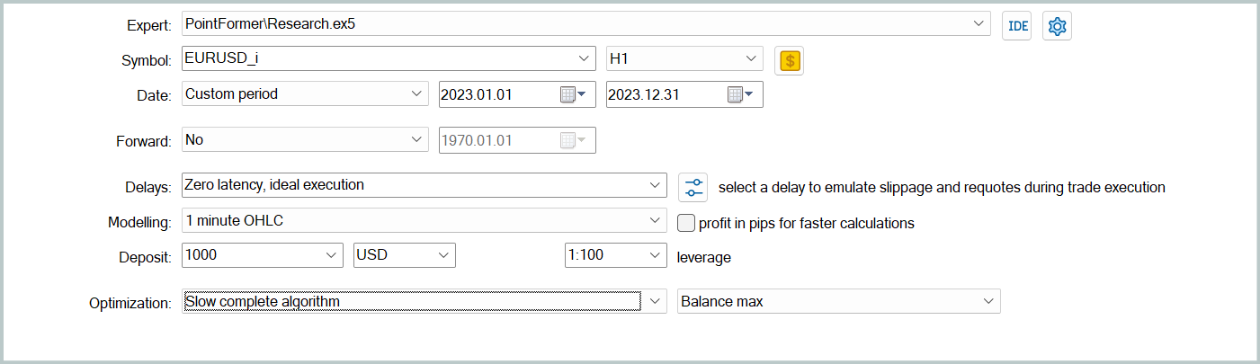
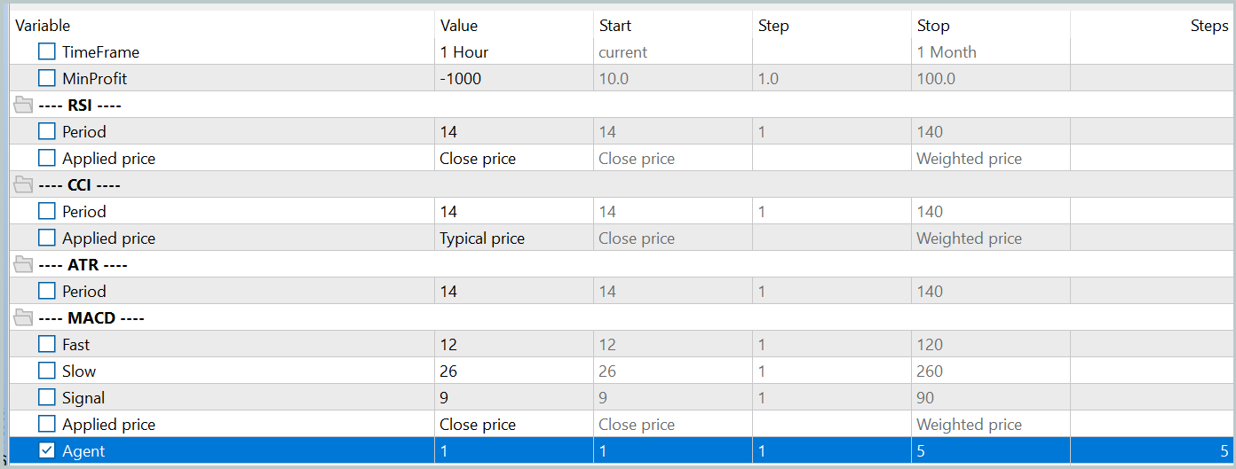
Now, it's time to examine the results of our implementation. As in previous work, we trained the models using real historical data from EURUSD for the year 2023, with the H1 timeframe. All indicator parameters were set to their default values.
Initially, we performed iterative offline training of the models by running the Expert Advisor "...\PointFormer\Study.mq5" in real-time mode. This EA does not perform any trading operations. Its logic is solely focused on training the models.
The first training iterations are performed on data collected during the model training processes from previous studies. The structure and parameters of the training data remained unchanged.
We then update the training dataset to better reflect the current action policy of the Actor. This allows for more accurate evaluation of its behavior during training and enables better adjustments to the policy optimization direction. For this, we launch a slow optimization mode in the Strategy Tester, using the environment interaction Expert Advisor "...\PointFormer\Research.mq5".
After that, we repeat the model training process.
The training of models and the updating of the training dataset are performed iteratively over several cycles. A good indication that training can be concluded is the achievement of acceptable results across all passes of the final iteration of dataset updates.
It is worth noting that minor discrepancies in the outcomes of individual passes are permissible. This is due to the use of a stochastic policy by the Actor, which naturally involves some randomness in actions within the learned behavioral range. As the models continue training, this stochastic behavior typically decreases. However, some variability in actions remains acceptable, if it does not significantly affect the overall profitability of the policy.
After several iterations of model training and dataset updates, we succeeded in obtaining a policy that is capable of generating profit on both the training and test datasets.
We evaluated the performance of the trained model using the MetaTrader 5 Strategy Tester, running tests on historical data from January 2024, while keeping all other parameters unchanged. The test results are presented below.
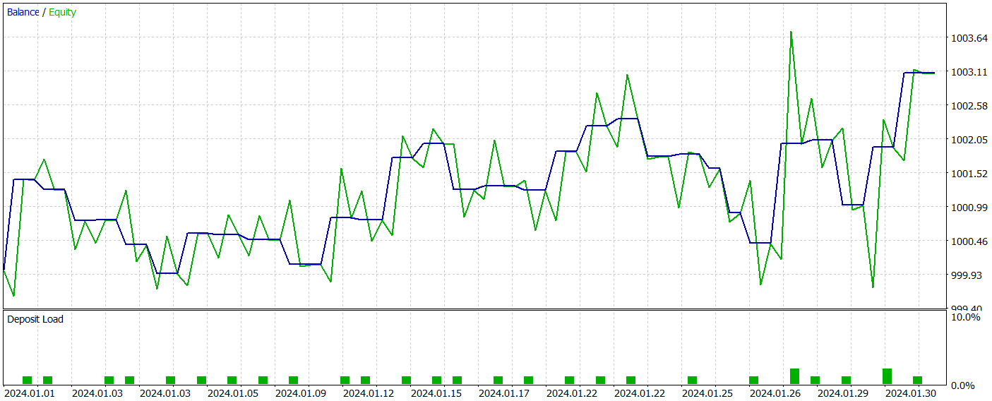
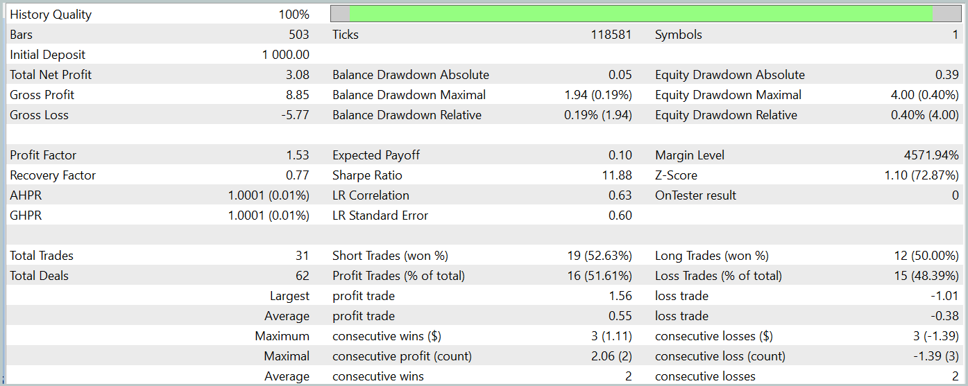
During the test period, the trained model executed a total of 31 trading operations, half of which were closed in profit. Notably, a nearly 50% higher value in maximum and average profitable trades compared to their losing counterparts led to a profit factor of 1.53. Despite the upward trend observed in the equity curve, the limited number of trades prevents us from drawing any definitive conclusions about the model’s effectiveness over a longer time horizon.
Conclusion
In this article, we explored the Pointformer method, which introduces a new architecture for working with point cloud data. The proposed algorithm combines local and global Transformers, enabling the effective extraction of both local and global spatial patterns from multidimensional data. Pointformer uses attention mechanisms to process information with respect to spatial context, and it supports learning while accounting for the relative importance of each point.
In the practical part of the article, we implemented our vision of the proposed approaches in the MQL5 language. We trained and tested the model based on the described algorithms. And the results demonstrate the method's potential for analyzing complex data structures.
That said, it is important to acknowledge that further research and optimization are required to gain a fuller understanding of Pointformer capabilities in the context of financial data analysis.
References
Programs used in the article
| # | Issued to | Type | Description |
|---|---|---|---|
| 1 | Research.mq5 | Expert Advisor | EA for collecting examples |
| 2 | ResearchRealORL.mq5 | Expert Advisor | EA for collecting examples using the Real-ORL method |
| 3 | Study.mq5 | Expert Advisor | Model training EA |
| 4 | Test.mq5 | Expert Advisor | Model testing EA |
| 5 | Trajectory.mqh | Class library | System state description structure |
| 6 | NeuroNet.mqh | Class library | A library of classes for creating a neural network |
| 7 | NeuroNet.cl | Library | OpenCL program code library |
Translated from Russian by MetaQuotes Ltd.
Original article: https://www.mql5.com/ru/articles/15820
- Free trading apps
- Over 8,000 signals for copying
- Economic news for exploring financial markets
You agree to website policy and terms of use
on historical data from January 2024.
Why only January, isn't it already September? Or is it implied that one has to retrain every month?
Why only January, is it already September? Or is it implied that one has to retrain every month?
You can't train a model on 1 year of data and expect stable performance over the same or longer time frame. To get stable model performance for 6-12 months, you need a much longer history to train. Consequently, it will take more time and cost to train the model.