Data Science and ML (Part 28): Predicting Multiple Futures for EURUSD, Using AI

MetaTrader 5 — Trading | 1 August 2024, 17:40

215

Omega J Msigwa

Contents

Introduction

In the world of financial data analysis using machine learning, the goal is often to predict future values based on historical data. While predicting the next immediate value is very useful as we discussed in many articles of this series. There are many situations in real-world applications where we might need to predict multiple future values instead of one. The attempt to predict various consecutive values is known as Multi-step or Multi-horizon forecasting.

Multi-step forecasting is crucial in various domains, such as finance, weather prediction, supply chain management, and healthcare. For instance, in financial markets, investors need to forecast stock prices or exchange rates for several days, weeks, or even months ahead. In weather prediction, accurate forecasts for the upcoming days or weeks can help in planning and disaster management.

This article assumes you have a basic understanding of machine learning and AI, ONNX, How to Use ONNX models in MQL5, Linear Regression, LightGBM, and Neural Networks.

The process of multistep forecasting involves several methodologies, each with its strengths and weaknesses. These methods include.

Direct multistep forecasting
Recursive multistep forecasting
Multi-output models
Vector Auto-regression (VAR) (will be discussed in the next article(s))

In this article, we will explore these methodologies, their applications, and how they can be implemented using various machine learning and statistical techniques. By understanding and applying multistep forecasting, we can make more informed decisions about the future of EURUSD.

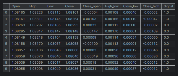
# Create target variables for multiple future steps

def create_target(df, future_steps=10):
    target = pd.concat([df['Close'].shift(-i) for i in range(1, future_steps + 1)], axis=1) # using close prices for the next i bar
    target.columns = [f'target_close_{i}' for i in range(1, future_steps + 1)] # naming the columns
    return target

# Combine features and targets

new_df = pd.DataFrame({
    'Open': df['Open'],
    'High': df['High'],
    'Low': df['Low'],
    'Close': df['Close']
})


future_steps = 5

target_columns = create_target(new_df, future_steps).dropna()
combined_df = pd.concat([new_df, target_columns], axis=1) #concatenating the new pandas dataframe with the target columns

combined_df = combined_df.dropna() #droping rows with NaN values caused by shifting values

target_cols_names = [f'target_close_{i}' for i in range(1, future_steps + 1)]

X = combined_df.drop(columns=target_cols_names).values #dropping all target columns from the x array
y = combined_df[target_cols_names].values # creating the target variables

print(f"x={X.shape} y={y.shape}")
combined_df.head(10)

Direct Multistep Forecasting

Direct multistep forecasting is a method where separate predictive models are trained for each future timestep you want to predict. For example, If we to predict the values for the next 5 timesteps, we would train 5 different models. One to predict the first step, another to predict the second step, and so on.

In direct multistep forecasting, each model is designed to predict a specific horizon. This approach allows each model to focus on the specific patterns and relationships that are relevant to its corresponding future timestep, potentially improving the accuracy of each prediction. However, it also means that you need to train and maintain multiple models, which can be resource-intensive.

Let us attempt multistep forecasting using the LightGBM machine learning model.

Firstly, we create a function to handle data from multiple steps.

Preparing the data

Python code

def multi_steps_data_process(data, step, train_size=0.7, random_state=42):

    # Since we are using the OHLC values only
    
    data["next signal"] = data["Signal"].shift(-step) # The target variable from next n future values
    data = data.dropna()
        
    y = data["next signal"]
    X = data.drop(columns=["Signal", "next signal"])
    
    return train_test_split(X, y, train_size=train_size, random_state=random_state)

This function creates the new target variable using the column "Signal" from the dataset. The target variable is taken from the index step+1 value in the signal column.

Suppose you have.

Signals
1
2
3
4
5

At step 1, the next signal will be 2, at step 2, the next signal will be 3, and so on.

This means that in step 1, we create a dataset in such a way the target variable is a value from 1 bar in the future, and so on. All the independent variables remain the same.

In this article, we are going to use data taken from the Hourly timeframe on EURUSD for 1000 bars.

Python code

df = pd.read_csv("/kaggle/input/eurusd-period-h1/EURUSD.PERIOD_H1.csv")

print(df.shape)
df.head(10)

Outputs

For simplicity, I created a mini dataset for five(5) variables only.

The "Signal" column represents bullish or bearish candle signals, it was created by the logic, that whenever the Close price was greater than the open price the signal was assigned a value of 1 and assigned a value of 0 for the opposite.

Now that we have a function to create multisteps data, Let us declare our models for handling each step.

Training Multiple Models for Forecasting

Hard-coding the models for each timestep manually could be time-consuming and ineffective, Coding within a loop will be easier and more effective. Within the loop, we do all the necessary things such as, training, validating, and saving the model for external use in MetaTrader 5.

Python code

for pred_step in range(1, 6): # We want to 5 future values

    lgbm_model = lgbm.LGBMClassifier(**params)
    
    
    X_train, X_test, y_train, y_test = multi_steps_data_process(new_df, pred_step) # preparing data for the current step
    
    
    lgbm_model.fit(X_train, y_train) # training the model for this step
    
    # Testing the trained mdoel 
    
    test_pred = lgbm_model.predict(X_test) # Changes from bst to pipe
 
        
    # Ensuring the lengths are consistent

    if len(y_test) != len(test_pred):
        test_pred = test_pred[:len(y_test)]
        
    
    print(f"model for next_signal[{pred_step} accuracy={accuracy_score(y_test, test_pred)}")
    
    #  Saving the model in ONNX format, Registering ONNX converter

    update_registered_converter(
        lgbm.LGBMClassifier,
        "GBMClassifier",
        calculate_linear_classifier_output_shapes,
        convert_lightgbm,
        options={"nocl": [False], "zipmap": [True, False, "columns"]},
    )
    # Final LightGBM conversion to ONNX

    model_onnx = convert_sklearn(
        lgbm_model,
        "lightgbm_model",
        [("input", FloatTensorType([None, X_train.shape[1]]))],
        target_opset={"": 12, "ai.onnx.ml": 2},
    )

    # And save.
    with open(f"lightgbm.EURUSD.h1.pred_close.step.{pred_step}.onnx", "wb") as f:
        f.write(model_onnx.SerializeToString())

Outputs

model for next_signal[1 accuracy=0.5033333333333333
model for next_signal[2 accuracy=0.5566666666666666
model for next_signal[3 accuracy=0.4866666666666667
model for next_signal[4 accuracy=0.4816053511705686
model for next_signal[5 accuracy=0.5317725752508361

Surprisingly, the model for forecasting the next second bar was the most accurate model, With an accuracy of 55% followed by the model for predicting the next fifth(5th) bar which provided a 53% accuracy.

Loading Models for Forecasting in MetaTrader 5

We start by integrating all the LightGBM AI models saved in ONNX format inside our Expert Advisor as resource files.

MQL5 code

#resource "\\Files\\lightgbm.EURUSD.h1.pred_close.step.1.onnx" as uchar model_step_1[]
#resource "\\Files\\lightgbm.EURUSD.h1.pred_close.step.2.onnx" as uchar model_step_2[]
#resource "\\Files\\lightgbm.EURUSD.h1.pred_close.step.3.onnx" as uchar model_step_3[]
#resource "\\Files\\lightgbm.EURUSD.h1.pred_close.step.4.onnx" as uchar model_step_4[]
#resource "\\Files\\lightgbm.EURUSD.h1.pred_close.step.5.onnx" as uchar model_step_5[]

#include <MALE5\Gradient Boosted Decision Trees(GBDTs)\LightGBM\LightGBM.mqh>

CLightGBM *light_gbm[5]; //for storing 5 different models
MqlRates rates[];

We then initialize our 5 different models.

MQL5 code

int OnInit()
  {
//---

   for (int i=0; i<5; i++)
     light_gbm[i] = new CLightGBM(); //Creating LightGBM objects

//---
   
   if (!light_gbm[0].Init(model_step_1))
     {
       Print("Failed to initialize model for step=1 predictions");
       return INIT_FAILED;
     }
   
   if (!light_gbm[1].Init(model_step_2))
     {
       Print("Failed to initialize model for step=2 predictions");
       return INIT_FAILED;
     }
   
   if (!light_gbm[2].Init(model_step_3))
     {
       Print("Failed to initialize model for step=3 predictions");
       return INIT_FAILED;
     }
   
   if (!light_gbm[3].Init(model_step_4))
     {
       Print("Failed to initialize model for step=4 predictions");
       return INIT_FAILED;
     }
   
   if (!light_gbm[4].Init(model_step_5))
     {
       Print("Failed to initialize model for step=5 predictions");
       return INIT_FAILED;
     }
      
   
   return(INIT_SUCCEEDED);
  }

Finally, we can collect Open, High, Low, and Close values from the previous bar and use them to get predictions from all 5 different models.

MQL5 code

void OnTick()
  {
//---
   
   CopyRates(Symbol(), PERIOD_H1, 1, 1, rates);
   vector input_x = {rates[0].open, rates[0].high, rates[0].low, rates[0].close};
   
   string comment_string = "";
   int signal = -1;
   
   for (int i=0; i<5; i++)
    {
      signal = (int)light_gbm[i].predict_bin(input_x);
      comment_string += StringFormat("\n Next[%d] bar predicted signal=%s",i+1, signal==1?"Buy":"Sell");
    }
    
   Comment(comment_string);
  }

Outcome

Strengths of Direct Multistep Forecasting

Each model is specialized for a particular forecast horizon, potentially leading to more accurate predictions for each step.
Training separate models can be straightforward, especially if you are using simple machine learning algorithms.
You can choose different models or algorithms for each step, allowing for greater flexibility in handling different forecasting challenges.

Weaknesses of Direct Multstep Forecasting

It requires training and maintaining multiple models, which can be computationally expensive and time-consuming.
Unlike recursive methods, errors from one step do not directly propagate to the next, which can be both a strength and a weakness. It can lead to inconsistency between steps.
Each model is independent and may not capture the dependencies between forecast horizons as effectively as a unified approach.

Recursive Multistep Forecasting

Recursive multistep forecasting, also known as iterative forecasting, is a method where a single model is used to make a one-step-ahead prediction. This prediction is then fed back into the model to make the next prediction. This process is repeated until predictions are made for the desired number of future timesteps.

In recursive multistep forecasting, the model is trained to predict the next immediate value. Once this value is predicted, it is added to the input data and used to predict the next value. This method leverages the same model iteratively.

To achieve this we are going to use the Linear Regression model to predict the next closing price using the previous close, This way the predicted close price can be used as the input for the next iteration and so on. This approach seems to be working well as easily with a single independent variable(feature).

Python code

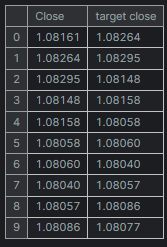
new_df = pd.DataFrame({
    'Close': df['Close'],
    'target close': df['Close'].shift(-1) # next bar closing price
})

Then.

new_df = new_df.dropna() # after shifting we want to drop all NaN values

X = new_df[["Close"]].values # Assigning close values into a 2D x array
y = new_df["target close"].values

print(new_df.shape)
new_df.head(10)

Outputs

Training & Testing a Linear Regression Model

Before training the model, we split the data without randomizing. This could help the model capture temporal dependencies between the values, as we know the next close is affected by the previous close price.

model = Pipeline([
    ("scaler", StandardScaler()),
    ("linear_regression", LinearRegression())
])


# Split the data into training and test sets

train_size = int(len(new_df) * 0.7)
X_train, X_test = X[:train_size], X[train_size:]
y_train, y_test = y[:train_size], y[train_size:]

# Train the model
model.fit(X_train, y_train)

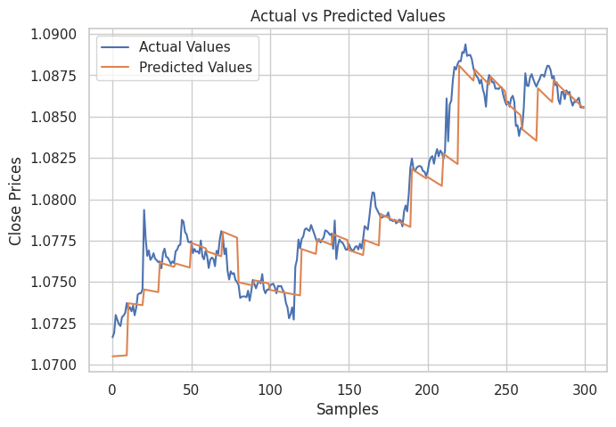
I then created a plot for showing the actual values from the testing sample and their predicted values, for analyzing how effective the model was in making predictions.

# Testing the Model

test_pred = model.predict(X_test) # Make predictions on the test set

# Plot the actual vs predicted values
plt.figure(figsize=(7.5, 5))
plt.plot(y_test, label='Actual Values')
plt.plot(test_pred, label='Predicted Values')
plt.xlabel('Samples')
plt.ylabel('Close Prices')
plt.title('Actual vs Predicted Values')
plt.legend()
plt.show()

Outcome

As can be seen from the image above. The model made decent predictions indeed, it was 98% accurate on the testing sample however, the predictions from the chart are how the linear model performed on the historical dataset, making predictions in a normal way not in a recursive format. To get the model to make recursive predictions we need to create a custom function for the work.

Python code

# Function for recursive forecasting
def recursive_forecast(model, initial_value, steps):
    predictions = []
    current_input = np.array([[initial_value]])
    
    for _ in range(steps):
        prediction = model.predict(current_input)[0]
        predictions.append(prediction)
        
        # Update the input for the next prediction
        current_input = np.array([[prediction]])
    
    return predictions

We can then obtain future predictions for 10 bars.

current_close = X[-1][0]  # Use the last value in the array

# Number of future steps to forecast
steps = 10

# Forecast future values
forecasted_values = recursive_forecast(model, current_close, steps)

print("Forecasted Values:")
print(forecasted_values)

Outputs

Forecasted Values:
[1.0854623040804965, 1.0853751608200348, 1.0852885667357617, 1.0852025183667728, 1.0851170122739744, 1.085032045039946, 1.0849476132688034, 1.0848637135860637, 1.0847803426385094, 1.0846974970940555]

To test the accuracy of a recursive model, we can use the function recursive_forecast above, to make predictions for the 10 next time steps throughout history from the current index after 10 timesteps in a loop.

predicted = []

for i in range(0, X_test.shape[0], steps):
    
    current_close = X_test[i][0]  # Use the last value in the test array
    
    forecasted_values = recursive_forecast(model, current_close, steps)
    predicted.extend(forecasted_values)
    
print(len(predicted))

Outputs

The recursive model accuracy was 91%.

Finally, we can save the Linear regression model to ONNX format that is compatible with MQL5.

# Convert the trained pipeline to ONNX
initial_type = [('float_input', FloatTensorType([None, 1]))]
onnx_model = convert_sklearn(model, initial_types=initial_type)

# Save the ONNX model to a file
with open("Lr.EURUSD.h1.pred_close.onnx", "wb") as f:
    f.write(onnx_model.SerializeToString())

print("Model saved to Lr.EURUSD.h1.pred_close.onnx")

Making Recursive Predictions in MQL5.

We start by adding the Linear Regression ONNX model in our Expert Advisor.

#resource "\\Files\\Lr.EURUSD.h1.pred_close.onnx" as uchar lr_model[]

We then import the Linear Regression model handler class.

#include <MALE5\Linear Models\Linear Regression.mqh>
CLinearRegression lr;

After initializing the model inside the OnInit function, We can get the previous closed bar close price, and then make predictions for the next 10 bars.

int OnInit()
  {
//---
   
   if (!lr.Init(lr_model))
     return INIT_FAILED;
   
//---
   
   ArraySetAsSeries(rates, true);

   return(INIT_SUCCEEDED);
  }
//+------------------------------------------------------------------+
//| Expert tick function                                             |
//+------------------------------------------------------------------+
void OnTick()
  {
//---
   
   CopyRates(Symbol(), PERIOD_H1, 1, 1, rates);
   vector input_x = {rates[0].close}; //get the previous closed bar close price
   
   vector predicted_close(10); //predicted values for the next 10 timestepps
   
   for (int i=0; i<10; i++)
    {
      predicted_close[i] = lr.predict(input_x);
      input_x[0] = predicted_close[i]; //The current predicted value is the next input
    }
   
   Print(predicted_close);
  }

Outputs

OR      0       16:39:37.018    Recursive-Multi step forecasting (EURUSD,H4)    [1.084011435508728,1.083933353424072,1.083855748176575,1.083778619766235,1.083701968193054,1.083625793457031,1.083550095558167,1.08347487449646,1.083400130271912,1.083325862884521]

To make things interesting, I decided to create trend-line objects to show these predicted values for 10 timesteps on the main chart.

   if (NewBar())
    {
      for (int i=0; i<10; i++)
       {
         predicted_close[i] = lr.predict(input_x);
         input_x[0] = predicted_close[i]; //The current predicted value is the next input
        
        //---
        
            ObjectDelete(0, "step"+string(i+1)+"-prediction"); //delete an object if it exists
            TrendCreate("step"+string(i+1)+"-prediction",rates[0].time, predicted_close[i], rates[0].time+(10*60*60), predicted_close[i], clrBlack); //draw a line starting from the previous candle to 10 hours forward
       }
    }

The TrendCreate function creates a short horizontal trendline starting from the previous closed bar to 10 bars forward.

Outcome

Advantages of Recursive Multistep Forecasting

Since only one model is trained and maintained, this simplifies the implementation and reduces computational resources.
Since the same model is used iteratively, it maintains consistency across the prediction horizon.

Weaknesses of Recursive Multistep Forecasting

Errors in early predictions can propagate and magnify in subsequent predictions, potentially reducing overall accuracy.
This approach assumes that the relationships captured by the model remain stable over the forecast horizon, which may not always be the case.

Multistep Forecasting Using Multi-output Models

Multi-output models are designed to predict multiple values at a time, we can use this to our advantage by making the models predict future timesteps simultaneously. Instead of training separate models for each forecast horizon or using a single model recursively, a multi-output model has multiple outputs, each corresponding to a future timestep.

In a multi-output model, the model is trained to produce a vector of predictions in a single pass. This means the model learns to understand the relationships and dependencies between different future timesteps directly. This approach can be well implemented using neural networks as they are capable of producing multiple outputs.

Preparing dataset for a Multi-outputs Neural Network model

We have to prepare the target variables for all the timesteps we want our trained neural network model to be able to predict.

Python code

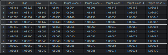
# Create target variables for multiple future steps

def create_target(df, future_steps=10):
    target = pd.concat([df['Close'].shift(-i) for i in range(1, future_steps + 1)], axis=1) # using close prices for the next i bar
    target.columns = [f'target_close_{i}' for i in range(1, future_steps + 1)] # naming the columns
    return target

# Combine features and targets

new_df = pd.DataFrame({
    'Open': df['Open'],
    'High': df['High'],
    'Low': df['Low'],
    'Close': df['Close']
})


future_steps = 5

target_columns = create_target(new_df, future_steps).dropna()
combined_df = pd.concat([new_df, target_columns], axis=1) #concatenating the new pandas dataframe with the target columns

combined_df = combined_df.dropna() #droping rows with NaN values caused by shifting values

target_cols_names = [f'target_close_{i}' for i in range(1, future_steps + 1)]

X = combined_df.drop(columns=target_cols_names).values #dropping all target columns from the x array
y = combined_df[target_cols_names].values # creating the target variables

print(f"x={X.shape} y={y.shape}")
combined_df.head(10)

Outputs

x=(995, 4) y=(995, 5)

Training and Testing Multi-outputs Neural Network

We start by defining a sequential neural network model.

Python code

# Defining the neural network model
model = Sequential([
    Input(shape=(X.shape[1],)),
    Dense(units = 256, activation='relu'),
    Dense(units = 128, activation='relu'),
    Dense(units = future_steps)
])

# Compiling the model
adam = Adam(learning_rate=0.01)
model.compile(optimizer=adam, loss='mse')

# Mmodel summary
model.summary()

Outputs

┏━━━━━━━━━━━━━━━━━━━━━━━━━━━━━━━━━┳━━━━━━━━━━━━━━━━━━━━━━━━┳━━━━━━━━━━━━━━━┓
┃ Layer (type)                    ┃ Output Shape           ┃       Param # ┃
┡━━━━━━━━━━━━━━━━━━━━━━━━━━━━━━━━━╇━━━━━━━━━━━━━━━━━━━━━━━━╇━━━━━━━━━━━━━━━┩
│ dense (Dense)                   │ (None, 256)            │         1,280 │
├─────────────────────────────────┼────────────────────────┼───────────────┤
│ dense_1 (Dense)                 │ (None, 128)            │        32,896 │
├─────────────────────────────────┼────────────────────────┼───────────────┤
│ dense_2 (Dense)                 │ (None, 5)              │           645 │
└─────────────────────────────────┴────────────────────────┴───────────────┘
 Total params: 34,821 (136.02 KB)
 Trainable params: 34,821 (136.02 KB)
 Non-trainable params: 0 (0.00 B)

We then split the data into training and testing samples respectively, unlike what we did in recursive multistep forecasting. This time we split the data after randomizing it with a 42 random seed since we don't want the model to understand sequential patterns as we believe the neural network will perform even better in understanding non-linear relationships from this data.

Finally, we train the NN model using the training data.

# Split the data into training and test sets
X_train, X_test, y_train, y_test = train_test_split(X, y, train_size=0.7, random_state=42)

scaler = MinMaxScaler()

X_train = scaler.fit_transform(X_train)
X_test = scaler.transform(X_test)

# Training the model

early_stopping = EarlyStopping(monitor='val_loss', patience=5, restore_best_weights=True) # stop training when 5 epochs doesn't improve

history = model.fit(X_train, y_train, epochs=20, validation_split=0.2, batch_size=32, callbacks=[early_stopping])

After testing the model on a test dataset.

# Testing the Model

test_pred = model.predict(X_test) # Make predictions on the test set

# Plotting the actual vs predicted values for each future step
plt.figure(figsize=(7.5, 10))
for i in range(future_steps):
    plt.subplot((future_steps + 1) // 2, 2, i + 1)  # subplots grid 
    plt.plot(y_test[:, i], label='Actual Values')
    plt.plot(test_pred[:, i], label='Predicted Values')
    plt.xlabel('Samples')
    plt.ylabel(f'Close Price +{i+1}')
    plt.title(f'Actual vs Predicted Values (Step {i+1})')
    plt.legend()

plt.tight_layout()
plt.show()

# Evaluating the model for each future step
for i in range(future_steps):
    accuracy = r2_score(y_test[:, i], test_pred[:, i])
    print(f"Step {i+1} - R^2 Score: {accuracy}")

Below is the outcome.

Step 1 - R^2 Score: 0.8664635514027637
Step 2 - R^2 Score: 0.9375671150885528
Step 3 - R^2 Score: 0.9040736780305894
Step 4 - R^2 Score: 0.8491904738263638
Step 5 - R^2 Score: 0.8458062142647863

The neural network produced impressive results for this regression problem. The code below shows how to obtain the predictions in Python.

# Predicting multiple future values

current_input = X_test[0].reshape(1, -1) # use the first row of the test set, reshape the data also
predicted_values = model.predict(current_input)[0] # adding[0] ensures we get a 1D array instead of 2D

print("Predicted Future Values:")
print(predicted_values)

Outputs

1/1 ━━━━━━━━━━━━━━━━━━━━ 0s 21ms/step
Predicted Future Values:
[1.0892788 1.0895394 1.0892794 1.0883198 1.0884078]

Then we can save this neural network model into ONNX format and the scaler files in binary formatted files.

import tf2onnx

# Convert the Keras model to ONNX
spec = (tf.TensorSpec((None, X_train.shape[1]), tf.float16, name="input"),)
model.output_names=['output']

onnx_model, _ = tf2onnx.convert.from_keras(model, input_signature=spec, opset=13)

# Save the ONNX model to a file
with open("NN.EURUSD.h1.onnx", "wb") as f:
    f.write(onnx_model.SerializeToString())
    
# Save the used scaler parameters to binary files

scaler.data_min_.tofile("NN.EURUSD.h1.min_max.min.bin")
scaler.data_max_.tofile("NN.EURUSD.h1.min_max.max.bin")

Finally, We can use the saved model and its data scaler parameters' in MQL5.

Getting Neural Network Multistep Predictions in MQL5

We start by adding the model and the Min-max scaler parameters to our Expert Advisor(EA).

#resource "\\Files\\NN.EURUSD.h1.onnx" as uchar onnx_model[]; //rnn model in onnx format
#resource "\\Files\\NN.EURUSD.h1.min_max.max.bin" as double min_max_max[];
#resource "\\Files\\NN.EURUSD.h1.min_max.min.bin" as double min_max_min[];

We then import the regression neural network ONNX class and the MinMax scaler library handler.

#include <MALE5\Neural Networks\Regressor Neural Nets.mqh>
#include <MALE5\preprocessing.mqh>

CNeuralNets nn;
MinMaxScaler *scaler;

We can then Initialize the NN model and the scaler, then obtain the final predictions from the model.

MqlRates rates[];
//+------------------------------------------------------------------+
//| Expert initialization function                                   |
//+------------------------------------------------------------------+
int OnInit()
  {
//---

   if (!nn.Init(onnx_model))
     return INIT_FAILED;
   
   scaler = new MinMaxScaler(min_max_min, min_max_max); //Initializing the scaler, populating it with trained values
   
//---
   
   ArraySetAsSeries(rates, true);
   
   return(INIT_SUCCEEDED);
  }
//+------------------------------------------------------------------+
//| Expert deinitialization function                                 |
//+------------------------------------------------------------------+
void OnDeinit(const int reason)
  {
//---
     if (CheckPointer(scaler)!=POINTER_INVALID)
       delete (scaler);
  }
//+------------------------------------------------------------------+
//| Expert tick function                                             |
//+------------------------------------------------------------------+
void OnTick()
  {
//---

   CopyRates(Symbol(), PERIOD_H1, 1, 1, rates);
   vector input_x = {rates[0].open, rates[0].high, rates[0].low, rates[0].close};
   input_x = scaler.transform(input_x); // We normalize the input data
   
   vector preds = nn.predict(input_x);
   
   Print("predictions = ",preds);
  }

Outputs

2024.07.31 19:13:20.785 Multi-step forecasting using Multi-outputs model (EURUSD,H4)    predictions = [1.080284595489502,1.082370758056641,1.083482265472412,1.081504583358765,1.079929828643799]

To make matters interesting, I added Trendlines on the chart to mark all the neural network future predictions.

void OnTick()
  {
//---

   CopyRates(Symbol(), PERIOD_H1, 1, 1, rates);
   vector input_x = {rates[0].open, rates[0].high, rates[0].low, rates[0].close};
   
   if (NewBar())
    {
      input_x = scaler.transform(input_x); // We normalize the input data 
      vector preds = nn.predict(input_x);
      
      for (int i=0; i<(int)preds.Size(); i++)
       {  
        //---
        
            ObjectDelete(0, "step"+string(i+1)+"-prediction"); //delete an object if it exists
            TrendCreate("step"+string(i+1)+"-prediction",rates[0].time, preds[i], rates[0].time+(5*60*60), preds[i], clrBlack); //draw a line starting from the previous candle to 5 hours forward
       }
    }
  }

This time we got better-looking prediction lines than those we obtained using the recursive linear regression model.

Overview of Multistep Forecasting Using Multi-Output Models

Advantages

By predicting multiple steps at once, the model can capture the relationships and dependencies between future timesteps.
Only one model is needed, this simplifies implementation and maintenance.
The model learns to produce consistent predictions across the entire forecast horizon.

Disadvantages

Training a model to output multiple future values can be more complex and may require more sophisticated architectures, especially for neural networks.
Depending on the complexity of the model, it may require more computational resources for training and inference.
There is a risk of overfitting, especially if the forecast horizon is long and the model becomes too specialized to the training data.

Utilizing Multistep Forecasting in Trading Strategies

Multistep forecasting, especially using models like neural networks and LightGBM, can significantly enhance various trading strategies by enabling dynamic adjustments based on predicted market movements. In grid trading, rather than setting fixed orders, multistep forecasts allow for dynamic entries that adjust to anticipated price changes, improving the system's responsiveness to market conditions.

Hedging strategies also benefit as forecasts provide guidance on when to open or close positions to protect against potential losses, such as taking short positions or buying put options if a downward trend is predicted. Furthermore, in trend detection, understanding future market directions through forecasting helps traders align their strategies accordingly, either by favoring short positions or exiting long ones to avoid losses.

Lastly, in high-frequency trading (HFT), rapid multistep forecasts can guide algorithms to capitalize on short-term price movements, thus enhancing profitability by executing timely buy and sell orders based on the predicted price changes in the coming seconds or minutes.

The Bottom Line

In financial analysis and forex trading, having the ability to predict multiple values into the future is very useful as discussed in the prior section of this article. This post was aimed to provide you with different approaches on how to take on this challenge. In the next article(s) we are going to explore Vector Auto-Regression which is a technique built for the task of analyzing multiple values and can predict multiple values as well.

Peace out.

Track development of machine learning models and much more discussed in this article series on this GitHub repo.

Attachments Table

File name	File Type	Descriptions & Usage
Direct Muilti step Forecasting.mq5 Multi-step forecasting using multi-outputs model.mq5 Recursive-Multi step forecasting.mq5	Expert Advisors	This EA has the code that uses multiple LightGBM model for multisteps forecasting. This EA has the neural network model predicting multiple steps using multi-outputs structure. This EA has the Linear regression iteratively predicting future timesteps.
LightGBM.mqh	MQL5 library file	Has the code for loading the LightGBM model in ONNX format and use it to make predictions.
Linear Regression.mqh	MQL5 library file	Has the code for loading the Linear-regression model in ONNX format and use it for predictions.
preprocessing.mqh	MQL5 library file	This file consists of the MInMax scaler, a scalling technique used to normalize the input data.
Regressor Neural Nets.mqh	MQL5 library file	Has the code for loading and deploying the neural network model from ONNX format to MQL5.
lightgbm.EURUSD.h1.pred_close.step.1.onnx lightgbm.EURUSD.h1.pred_close.step.2.onnx lightgbm.EURUSD.h1.pred_close.step.3.onnx lightgbm.EURUSD.h1.pred_close.step.4.onnx lightgbm.EURUSD.h1.pred_close.step.5.onnx Lr.EURUSD.h1.pred_close.onnx NN.EURUSD.h1.onnx	AI models in ONNX format	LightGBM models for predicting the next future step values A simple linear regression model in ONNX format Feed forward Neural Network in ONNX format
NN.EURUSD.h1.min_max.max.bin NN.EURUSD.h1.min_max.min.bin	Binary Files	Contains maximum and minimum values respectively for the MIn-max scaler
predicting-multiple-future-tutorials.ipynb	Jupyter Notebook	All the python code shown in this article can be located in this file

Attached files |

Download ZIP

Attachments.zip (519.77 KB)

Warning: All rights to these materials are reserved by MetaQuotes Ltd. Copying or reprinting of these materials in whole or in part is prohibited.

Introduction

Direct Multistep Forecasting

Strengths of Direct Multistep Forecasting

Weaknesses of Direct Multstep Forecasting

Recursive Multistep Forecasting

Advantages of Recursive Multistep Forecasting

Weaknesses of Recursive Multistep Forecasting

Multistep Forecasting Using Multi-output Models

Overview of Multistep Forecasting Using Multi-Output Models

Utilizing Multistep Forecasting in Trading Strategies

The Bottom Line

Other articles by this author