Data Science and Machine Learning (Part 23): Why LightGBM and XGBoost outperform a lot of AI models?

MetaTrader 5 — Statistics and analysis | 30 May 2024, 13:54

2 522

Omega J Msigwa

What are Gradient Boosted Trees?

Gradient Boosted Decision Trees (GBDT) are a powerful machine learning technique used primarily for regression and classification tasks. They combine the predictions of multiple weak learners, usually decision trees, to create a strong predictive model.

The core idea is to build models sequentially, each new model attempting to correct the errors made by the previous ones.

These boosted trees such as:

Extreme Gradient Boosting (XGBoost): Which is a popular and efficient implementation of gradient boosting,
Light Gradient Boosting Machnine (LightGBM): Which was designed for high performance and efficiency, especially with large datasets.
CatBoost: Which Handles categorical features automatically and is robust against overfitting.

Have gained much popularity in the machine learning community as the algorithms of choice for many winning teams in machine learning competitions. In this article, we are going to discover how we can use these accurate models in our trading applications.

Key Concepts

Boosting

Boosting is an ensemble learning technique that combines multiple weak learners (models that perform slightly better than random guessing) to form a strong learner.
Each new model focuses on the mistakes of the previous models, gradually improving the overall performance.

Gradient Descent

Gradient boosting uses gradient descent to minimize a loss function, which is the difference between the predicted and actual values.
By iteratively adding new models that point in the direction of the gradient of the loss function, the ensemble model is refined.

With Just a few lines of code, these boosted trees not only can give you a reasonable accuracy but also can get your data science project to the next level.

import lightgbm as lgb

train_data = lgb.Dataset(X_train, label=y_train) # preparing data the lightgbm way
val_data = lgb.Dataset(X_test, label=y_test, reference=train_data)

params = {
    'boosting_type': 'gbdt',  # Gradient Boosting Decision Tree
    'objective': 'binary',  # For binary classification (use 'regression' for regression tasks)
    'metric': ['auc','binary_logloss'],  # Evaluation metric
    'num_leaves': 10,  # Number of leaves in one tree
    'n_estimators' : 100, # number of trees
    'max_depth': 5,
    'learning_rate': 0.05,  # Learning rate
    'feature_fraction': 0.9  # Fraction of features to be used for each boosting round
}

# Train the model with evaluation results stored
num_round = 100

bst = lgb.train(params, train_data, num_round, valid_sets=[train_data, val_data])


y_pred = bst.predict(X_test, num_iteration=bst.best_iteration)

# For binary classification, you might want to threshold the predictions
y_pred_binary = np.round(y_pred)


print("Classification Report\n",
      classification_report(y_test, y_pred_binary))

Results:

Classification Report
               precision    recall  f1-score   support

         0.0       0.70      0.75      0.73       104
         1.0       0.71      0.66      0.68        96

    accuracy                           0.70       200
   macro avg       0.71      0.70      0.70       200
weighted avg       0.71      0.70      0.70       200

I applied the same data other popular classifiers.

Classifier	Classification Report
Logistic Regression	precision recall f1-score support 0.0 0.69 0.76 0.72 104 1.0 0.71 0.62 0.66 96 accuracy 0.69 200 macro avg 0.70 0.69 0.69 200 weighted avg 0.70 0.69 0.69 200
Decision Tree	precision recall f1-score support 0.0 0.62 0.61 0.61 104 1.0 0.59 0.60 0.59 96 accuracy 0.60 200 macro avg 0.60 0.60 0.60 200 weighted avg 0.61 0.60 0.61 200
Naive Bayes	precision recall f1-score support 0.0 0.64 0.84 0.73 104 1.0 0.73 0.49 0.59 96 accuracy 0.67 200 macro avg 0.69 0.67 0.66 200 weighted avg 0.68 0.67 0.66 200
K-Nearest Neighbors	precision recall f1-score support 0.0 0.68 0.73 0.71 104 1.0 0.69 0.64 0.66 96 accuracy 0.69 200 macro avg 0.69 0.68 0.68 200 weighted avg 0.69 0.69 0.68 200
Support Vector Machine	precision recall f1-score support 0.0 0.69 0.69 0.69 104 1.0 0.66 0.66 0.66 96 accuracy 0.68 200 macro avg 0.67 0.67 0.67 200 weighted avg 0.67 0.68 0.67 200

The Light GBM model was the one with overall accuracy that the other classifiers for the same problem. You may have noticed that I did not even bother to normalize the input data but the model was stillable to outperform others. As we know normalization is crucial for machine learning models to perform but lightGBM seems to defy this idea. This is one of the things that make these models interesting.

Let us look at the difference between GBDT(LightGBM and XGBoost) and other machine learning classifiers.

Gradient Boosted Decision Trees (LighGBM & XGBoost) Vs Other Classifiers

LightGBM & XGBoost	Other Classifiers
They do not require feature scaling since they are based on decision trees which are insensitive to the scale of the input features.	Algorithms such as K-Nearest Neighbors(K-NN) and Support Vector Machine(SVM) which rely on distance between data points can not perform well on a dataset with features on different scales. Scaling is very important to most classifiers.
Both XGBoost and LightGBM have built-in mechanisms that can handle missing values. They can learn how to deal with missing data by assigning missing values to either side of a split during training or they can simply create a branch for that missing value in a tree and understand its pattern separately.	They can't handle missing values mostly. These missing values may lower accuracy.
Parameters tuning is important but not required; these models perform reasonably well with default parameters. Hyperparameters tuning is still crucial for achieving optimal performance.	Classifier Models like neural networks are very sensitive to hyperparameters. Default parameters won't help.

Now that we have seen how LightGBM and XGBoost fare against other machine learning classifiers let us dissect one model after the other, starting with XGBoost.

What is Extreme Gradient Boosting (XGBoost)?

XGBoost is an optimized distributed gradient boosting library designed for efficient and scalable training of machine learning models. Within it is an ensemble learning method that combines the predictions of multiple weak models to produce a stronger prediction.

How does XGBoost Work?

To understand how does XGBoost works lets understand its theory.

Initialization

It starts with an initial prediction, usually the mean of the target values for regression or the logarithm of the odds for classification.

Iterative Boosting

Residual Calculation: For each iteration , calculate the residuals (errors) of the predictions made by the current ensemble of models.

Where:

is the residual for the -th observation at iteration .

is the actual target value.

is the predicted value at iteration .

Fitting a New Tree: Fit a new decision tree to the residuals. The tree is built to predict the residuals of the current model.

The leaves of the tree represent the predicted adjustments to the current model's predictions.

Update the Model: Add the new tree’s predictions to the current model’s predictions, usually scaled by a learning rate .

Where:

is the prediction of the new tree at iteration for input .

Objective Function

The objective function in XGBoost consists of two parts:

The loss function, which measures how well the model fits the training data. Common loss functions include mean squared error for regression and log loss for classification.
The regularization term, which is responsible for penalizing the complexity of the model to prevent overfitting. XGBoost uses both L1 (Lasso) and L2 (Ridge) regularization.

The objective function to minimize is:

Where:

is the loss term.

Is the regularization term for the -th tree.

is the number of observations.

is the number of trees.

Gradient and Hessian

XGBoost uses second-order Taylor expansion (gradient and Hessian) to approximate the loss function for efficient computation of the optimal splits. The Gradient is the first derivative of the loss function with respect to the prediction while the Hessian is the second derivative of the loss function with respect to the prediction.

Trees Pruning

Trees are grown iteratively and pruned to optimize the objective function. Pruning helps prevent overfitting by removing nodes that do not provide a significant improvement in the objective function.

The learning rate η scales the contribution of each tree to control the step size in the boosting process. Smaller learning rates typically requires more trees.

Implementing XGBoost in Python

It takes a few lines of code to implement the XGBoost model in Python. Since it is a separate library you need to install it first if you haven't already.

pip install xgboost

We need to import the Pipeline function from Scikit-learn. This will help us make a machine learning object with pre-processing and other necessary steps.

from sklearn.pipeline import Pipeline

As said earlier boosted trees can perform well even without normalizing the data however, adding it won't hurt, not to mention it gives us several advantages such as helping us mitigate numerical instability issues caused by large numbers which might be a result of matrix multiplications in our models. Let us add the normalization as a good practice while we create a pipeline for the model and fit it to the training data.

Python:

# Create a pipeline with a scaler and the XGBoost classifier
pipe = Pipeline([
    ("scaler", StandardScaler()),
    ("xgb", xgb.XGBClassifier(**params))
])

# Fit the pipeline to the training data
pipe.fit(X_train, y_train)

The XGBoost model comes with some parameters that are crucial understanding not only how they work but also how you can tune them for the better.

Python:

params = {
    'objective': 'binary:logistic',  
    'learning_rate': 0.05,  
    'max_depth': 5,  
    'n_estimators': 100,  
    'colsample_bytree': 0.9,  
    'subsample': 0.9,  
    'eval_metric': ['auc', 'logloss']  
}

Parameter	Description	Tuning
objective	This parameter specifies the learning task and the corresponding learning objective, binary:logistic used above is used for binary classification with logistic regression. It gives out probability outputs.	Common objectives include 'reg:squarederror' for regression, 'binary:logistic' for binary classification, and 'multi:softmax' for multi-class classification. Always choose the objective based on the nature of your problem.
learning_rate	Also known as eta( ), this specifies the step size at each iteration while moving toward the minimum of the loss function. A lower learning rate makes the model robust by preventing overfitting but requires more boosting rounds and vice versa.	Lower learning rates (e.g., 0.01-0.1) tend to require more trees (higher n_estimators) but can improve model stability and performance. It is a good idea to start with a moderate value (e.g., 0.1) and adjust based on cross-validation performance.
max_depth	This is the maximum depth of the tree, Increasing this value makes the model more complex and more likely to overfit. It controls the complexity of the model, Deeper trees capture more patterns between features which increases the risk of overfitting.	Common values range from 3 to 10. Kindly use cross-validation to find the optimal depth.
n_estimators	This is the number of boosting rounds or trees to build. More trees increase computation time and are prone to overfit.	Early stopping can be used in cross-validation to find an appropriate number of trees.
colsample_bytree	It is the subsample ratio of columns when constructing each tree. A value of 0.9 ( used in the above code) means 90% of the features will be used to build each tree. Helps to reduce overfitting by introducing randomness at the column level. It can also speed up training and make the model more robust.	Values typically range from 0.3 to 1.0. Higher values use more features while lower values introduce more randomness.
subsample	The subsample ratio of the training instances. A value of 0.9 means 90% of the training data will be used to build each tree. Similar to colsample_bytree, this parameter reduces overfitting by adding randomness at the data level and can improve generalization.	Values typically range from 0.5 to 1.0. Higher values use more data while lower values introduce more randomness.
eval_metric	The evaluation metrics to be used during training. Multiple evaluation metrics can provide a more comprehensive view of model performance.	Common metrics include 'rmse' for regression, 'logloss' for classification, and 'error' for binary classification. Always choose metrics that align with your problem nature and goals.

Since we have already trained the model. Let us test it and observe its performance.

Python:

y_pred = pipe.predict(X_test) 

# For binary classification, you might want to threshold the predictions since these are probabilities
y_pred_binary = np.round(y_pred)

# Confusion Matrix
cm = confusion_matrix(y_test, y_pred_binary)
sns.heatmap(cm, annot=True, fmt='d', cmap='Blues')
plt.xlabel("Predicted Label")
plt.ylabel("True Label")
plt.title("Confusion Matrix")
plt.savefig("confusion-matrix xgboost")  # Display the heatmap


print("Classification Report\n",
      classification_report(y_test, y_pred_binary))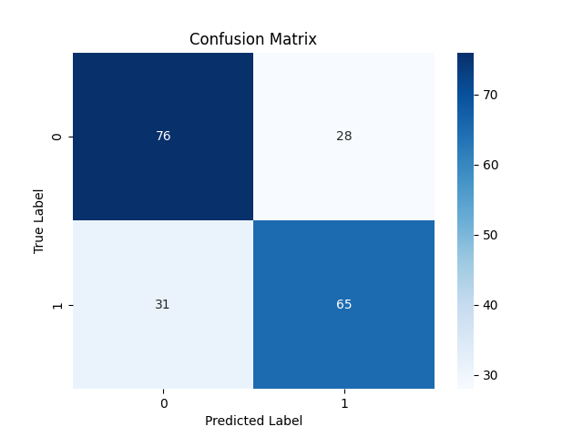

Confusion matrix:

confusion matrix xgboos.eurusd.h1

Classification Report
               precision    recall  f1-score   support

         0.0       0.71      0.73      0.72       104
         1.0       0.70      0.68      0.69        96

    accuracy                           0.70       200
   macro avg       0.70      0.70      0.70       200
weighted avg       0.70      0.70      0.70       200

The model did a great job on out-of-sample predictions, It was 71% and 70% accurate for bearish(class 0) and bullish(class 1) signals respectively.

Now that we have discussed XGBoost let us dissect LightGBM and see what it is all about.

What is Light Gradient Boosting Machine (LightGBM)?

This is an open-source machine learning framework specifically designed for efficiency, scalability, and accuracy. It was developed by Microsoft as a part of a distributed machine learning toolkit and was released on April 24th, 2017.

The LightGBM was built based on the existing Gradient Boosted Decision Trees such as XGBoost, It offers several key improvements outlined below.

Light GBM Improvements

Efficiency. LightGBM boasts significantly faster training speeds compared to XGBoost model. This is achieved through techniques like Gradient-based One-Side Sampling (GOSS) which focuses on data points with higher errors, reducing unnecessary computations.

Memory Usage. LightGBM utilizes histograms for efficient tree construction. This reduces memory consumption compared to other GBDT algorithms, making it particularly suitable for handling massive datasets that might not fit in memory with traditional approaches.

Scalability. LightGBM is designed for scalability. It can effectively handle large datasets due to its distributed learning capabilities. This allows training models on multiple machines in parallel, significantly speeding up the process for massive datasets.

Accuracy. While prioritizing speed and memory efficiency, LightGBM doesn't compromise on accuracy. The employed techniques are designed to achieve similar or even better performance compared to previous GBDT models.

How does LightGBM Work?

Light GBM works the same as XGBoost when it comes to mathematical theory with a slight change in how trees are grown, lets us look at the core concepts behind Light GBM.

Boosting. Same as XGBoost In gradient boosting, each new model aims to correct the errors made by the previous models by fitting to the residuals (errors).

Decision Trees. While XGBoost uses level-wise tree growth, meaning it grows the tree depth-wise and balances the tree more uniformly. LightGBM has leaf-wise tree growth, which can create deeper and more complex trees.

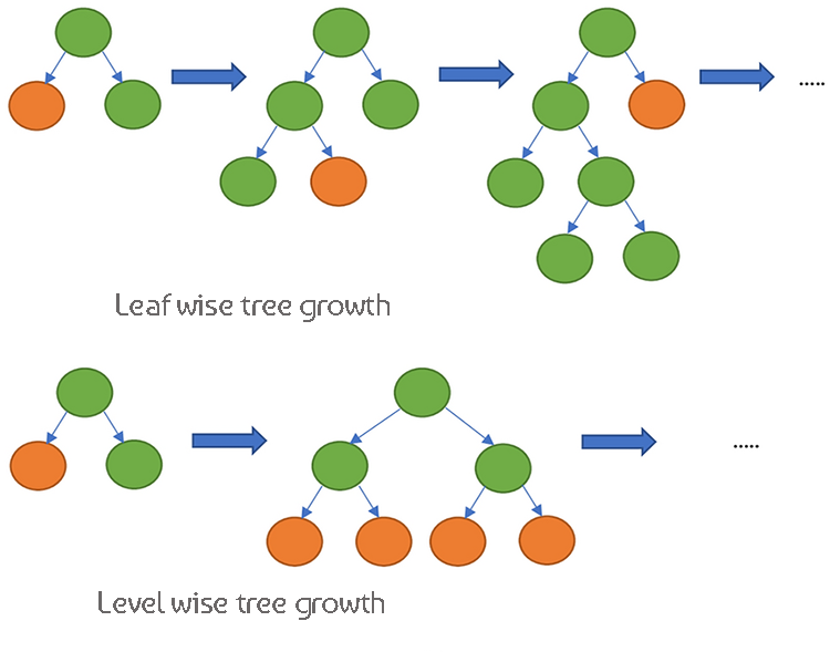
leaf wise vs level wise decision-tree growth

Since these two models are very similar in how they work, let us see their table of differences to help us understand them well by comparison.

The differences between XGBoost and Light GBM

Aspect	XGBoost	LightGBM
Tree Growth Strategy	Level-wise growth (grows trees depth-wise, more balanced trees)	Leaf-wise growth (grows the leaf with the highest loss reduction first, potentially deeper trees)
Handling Missing Values	Learns the optimal direction to handle missing values during training	Can handle missing values directly, splits data into non-missing and missing categories
Regularization	Uses L1 (Lasso) and L2 (Ridge) regularization to penalize model complexity	It Uses L2 regularization, focusing more on preventing overfitting
Sampling Technique	Uses traditional gradient boosting with all data	Gradient-based One-Side Sampling (GOSS) to focus on important data points with large gradients
Feature Handling	Requires one-hot encoding or other preprocessing for categorical variables	Supports categorical features natively using Exclusive Feature Bundling (EFB)
Sparsity Awareness	Optimized for sparse data, uses a sparsity-aware algorithm for memory and computation efficiency	Handles sparse data efficiently, it has similar optimization techniques as XGBoost
Split Finding Algorithm	Uses approximate algorithms and quantile sketches for efficient split finding by default	Uses histogram-based algorithms for faster split finding and memory efficiency
Parallel Processing	Supports parallel and distributed computing for large-scale data processing	Also supports parallel and distributed computing, optimized for large datasets
Training Speed	Generally slower compared to LightGBM due to level-wise growth	Generally faster due to leaf-wise growth and efficient sampling techniques
Flexibility and Customization	Highly flexible, supports custom loss functions and evaluation metrics	Also highly flexible, with extensive customization options for the boosting process

Implementing Light GBM in Python

As seen earlier it takes a few lines of code to implement a Light GBM model. Let us implement it this time within a pipeline. The same way we did with XGBoost.

We have to install it first.

pip install lightgbm

Light GBM also has some parameters that are important to understand.

Parameter	Description	Tuning
boosting_type	Type of boosting algorithm to use. The default is 'gbdt' (Gradient Boosting Decision Tree).	Typical values are 'gbdt', 'dart', 'goss'. 'gbdt' is the most common. Choose based on your dataset and experimentation.
objective	Specifies the learning task and the corresponding learning objective. 'binary' is used for binary classification.	Common objectives include 'regression' for regression tasks, 'binary' for binary classification. Always choose based on the nature of your problem.
metric	Evaluation metric(s) to be used during training. 'auc' and 'binary_logloss' are common for binary classification.	Typical values range from 20 to 50. Increasing num_leaves can capture more complex patterns but may lead to overfitting. Use cross-validation to find the optimal value.
num_leaves	Maximum number of leaves in one tree. A higher value increases model complexity and viceversa.	Typical values range from 20 to 50. Increasing this value can capture more complex patterns but may lead to overfitting.
n_estimators	Number of boosting rounds (trees). More trees generally increase computation time and the risk of overfitting.	Use early stopping in cross-validation to determine the appropriate number of trees. Start with a moderate value (e.g., 100) and adjust based on performance.
max_depth	Maximum depth of a tree. Increasing this value makes the model more complex and likely to overfit.	Common values range from 3 to 10. Deeper trees capture more patterns but increase the risk of overfitting. Use cross-validation to find the optimal depth.
learning_rate	Step size at each iteration while moving toward the minimum of the loss function. Lower values make the model more robust but require more boosting rounds.	Lower learning rates (e.g., 0.01-0.1) require more trees (higher n_estimators) but can improve model stability and performance. Start with a moderate value (e.g., 0.1) and adjust based on cross-validation performance.
feature_fraction	Fraction of features to be used for each boosting round. A value of 0.9 means 90% of the features will be used to build each tree.	Values typically range from 0.3 to 1.0. Higher values use more features, while lower values introduce more randomness. Helps to reduce overfitting by introducing randomness at the feature level.

For more information regarding these hyperparameters refer to the documentation linked at the end of the article. Now, let us train the Light GBM model.

Python:

params = {
    'boosting_type': 'gbdt',  # Gradient Boosting Decision Tree
    'objective': 'binary',  # For binary classification (use 'regression' for regression tasks)
    'metric': ['auc','binary_logloss'],  # Evaluation metric
    'num_leaves': 25,  # Number of leaves in one tree
    'n_estimators' : 100, # number of trees
    'max_depth': 5,
    'learning_rate': 0.05,  # Learning rate
    'feature_fraction': 0.9  # Fraction of features to be used for each boosting round
}

pipe = Pipeline([
    ("scaler", StandardScaler()),
    ("lgbm", lgb.LGBMClassifier(**params))
])

# Fit the pipeline to the training data
pipe.fit(X_train, y_train)

Outputs console:

[LightGBM] [Warning] feature_fraction is set=0.9, colsample_bytree=1.0 will be ignored. Current value: feature_fraction=0.9
[LightGBM] [Warning] feature_fraction is set=0.9, colsample_bytree=1.0 will be ignored. Current value: feature_fraction=0.9
[LightGBM] [Info] Number of positive: 398, number of negative: 402
[LightGBM] [Info] Auto-choosing col-wise multi-threading, the overhead of testing was 0.000177 seconds.
You can set `force_col_wise=true` to remove the overhead.
[LightGBM] [Info] Total Bins 1594
[LightGBM] [Info] Number of data points in the train set: 800, number of used features: 8
[LightGBM] [Info] [binary:BoostFromScore]: pavg=0.497500 -> initscore=-0.010000
[LightGBM] [Info] Start training from score -0.010000
[LightGBM] [Warning] No further splits with positive gain, best gain: -inf
[LightGBM] [Warning] No further splits with positive gain, best gain: -inf
[LightGBM] [Warning] No further splits with positive gain, best gain: -inf
[LightGBM] [Warning] No further splits with positive gain, best gain: -inf
[LightGBM] [Warning] No further splits with positive gain, best gain: -inf

We can not understand its performance for now, let us give the trained model new data and observe the performance.

y_pred = pipe.predict(X_test) # Changes from bst to pipe

# For binary classification, you might want to threshold the predictions
y_pred_binary = np.round(y_pred)

# Confusion Matrix
cm = confusion_matrix(y_test, y_pred_binary)
sns.heatmap(cm, annot=True, fmt='d', cmap='Blues')
plt.xlabel("Predicted Label")
plt.ylabel("True Label")
plt.title("Confusion Matrix")
plt.savefig("confusion-matrix lightgbm")  # Display the heatmap


print("Classification Report\n",
      classification_report(y_test, y_pred_binary))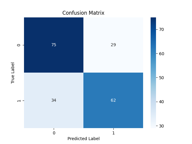

confusion matrix lightgbm

Classification Report
               precision    recall  f1-score   support

         0.0       0.69      0.72      0.70       104
         1.0       0.68      0.65      0.66        96

    accuracy                           0.69       200
   macro avg       0.68      0.68      0.68       200
weighted avg       0.68      0.69      0.68       200

Great, the model is 69% accurate on the testing sample, Now that we have these two well-trained models let us save both of them to ONNX format which we can deploy in MQL5.

Saving XGBoost and LightGBM to ONNX.

Saving these two models can be tricky since both of these models come separately in their custom libraries; Their saving process isn't straightforward-easy like saving Scikit-learn, TensorFlow, or Keras models. For more information kindly refer to ONNX documentation on how to save Light GBM and XGBoost.

Let us start by saving the Light GBM model, the process is the exact-same for both models.

Saving LightGBM model| Python code:

from skl2onnx.common.data_types import FloatTensorType
from skl2onnx import convert_sklearn, to_onnx, update_registered_converter
from skl2onnx.common.shape_calculator import calculate_linear_classifier_output_shapes
from onnxmltools.convert.xgboost.operator_converters.XGBoost import convert_xgboost
from onnxmltools.convert import convert_xgboost as convert_xgboost_booster

update_registered_converter(
    lgb.LGBMClassifier,
    "GBMClassifier",
    calculate_linear_classifier_output_shapes,
    convert_lightgbm,
    options={"nocl": [False], "zipmap": [True, False, "columns"]},
)

model_onnx = convert_sklearn(
    pipe,
    "pipeline_lightgbm",
    [("input", FloatTensorType([None, X_train.shape[1]]))],
    target_opset={"": 12, "ai.onnx.ml": 2},
)

# And save.
with open("lightgbm.eurusd.h1.onnx", "wb") as f:
    f.write(model_onnx.SerializeToString())

Saving XGBoost model | Python code:

update_registered_converter(
    xgb.XGBClassifier,
    "XGBClassifier",
    calculate_linear_classifier_output_shapes,
    convert_xgboost,
    options={"nocl": [False], "zipmap": [True, False, "columns"]},
)

model_onnx = convert_sklearn(
    pipe,
    "pipeline_xgboost",
    [("input", FloatTensorType([None, X_train.shape[1]]))],
    target_opset={"": 12, "ai.onnx.ml": 2},
)

# And save.
with open("xgboost.eurusd.h1.onnx", "wb") as f:
    f.write(model_onnx.SerializeToString())

Loading ONNX model in MQL5

Loading Gradient Boosted Decision Trees(GBDT) can be tricky unlike loading other models, despite the process being the same.

MQL5 | LightGBM.mqh

bool CLightGBM::OnnxLoad(long &handle)
 {
 
//--- since not all sizes defined in the input tensor we must set them explicitly
//--- first index - batch size, second index - series size, third index - number of series (only Close)
   
   OnnxTypeInfo type_info; //Getting onnx information for Reference In case you forgot what the loaded ONNX is all about

   long input_count=OnnxGetInputCount(handle);
   if (MQLInfoInteger(MQL_DEBUG))
      Print("model has ",input_count," input(s)");
   
   for(long i=0; i<input_count; i++)
     {
      string input_name=OnnxGetInputName(handle,i);
      if (MQLInfoInteger(MQL_DEBUG))
         Print(i," input name is ",input_name);
         
      if(OnnxGetInputTypeInfo(handle,i,type_info))
        {
          if (MQLInfoInteger(MQL_DEBUG))
            PrintTypeInfo(i,"input",type_info);
          ArrayCopy(inputs, type_info.tensor.dimensions);
        }
     }

   long output_count=OnnxGetOutputCount(handle);
   if (MQLInfoInteger(MQL_DEBUG))
      Print("model has ",output_count," output(s)");
      
   for(long i=0; i<output_count; i++)
     {
      string output_name=OnnxGetOutputName(handle,i);
      if (MQLInfoInteger(MQL_DEBUG))
         Print(i," output name is ",output_name);
         
      if(OnnxGetOutputTypeInfo(handle,i,type_info))
       {
         if (MQLInfoInteger(MQL_DEBUG))
            PrintTypeInfo(i,"output",type_info);
         ArrayCopy(outputs, type_info.tensor.dimensions);
       }
     }
   
//---
   
   replace(inputs);
   replace(outputs);
      
//--- Setting the input size

   for (long i=0; i<input_count; i++)   
     if (!OnnxSetInputShape(handle, i, inputs)) //Giving the Onnx handle the input shape
       {
         printf("Failed to set the input shape Err=%d",GetLastError());
         DebugBreak();
         return false;
       }
   
//--- Setting the output size
   
   for(long i=0; i<output_count; i++)
     {
      if(!OnnxSetOutputShape(handle,i,outputs))
       {
          printf("Failed to set the Output[%d] shape Err=%d",i,GetLastError());
          //DebugBreak();
          //return false;
       }
     }
     
   initialized = true;
   
   Print("ONNX model Initialized");
   return true;
 }

Outputs | Experts tab:

JM 0 10:49:34.197 LightGBM EA (EURUSD,H1) model has 1 input(s)

MG 0 10:49:34.197 LightGBM EA (EURUSD,H1) 0 input name is input

KM 0 10:49:34.198 LightGBM EA (EURUSD,H1) type ONNX_TYPE_TENSOR

CF 0 10:49:34.198 LightGBM EA (EURUSD,H1) data type ONNX_TYPE_TENSOR

HP 0 10:49:34.198 LightGBM EA (EURUSD,H1) shape [-1, 8]

EI 0 10:49:34.198 LightGBM EA (EURUSD,H1) 0 input shape must be defined explicitly before model inference

RN 0 10:49:34.198 LightGBM EA (EURUSD,H1) shape of input data can be reduced to [8] if undefined dimension set to 1

EM 0 10:49:34.198 LightGBM EA (EURUSD,H1) model has 2 output(s)

MJ 0 10:49:34.198 LightGBM EA (EURUSD,H1) 0 output name is output_label

MR 0 10:49:34.198 LightGBM EA (EURUSD,H1) type ONNX_TYPE_TENSOR

EI 0 10:49:34.198 LightGBM EA (EURUSD,H1) data type ONNX_TYPE_TENSOR

RK 0 10:49:34.198 LightGBM EA (EURUSD,H1) shape [-1]

RN 0 10:49:34.198 LightGBM EA (EURUSD,H1) 0 output shape must be defined explicitly before model inference

GJ 0 10:49:34.198 LightGBM EA (EURUSD,H1) 1 output name is output_probability

OR 0 10:49:34.198 LightGBM EA (EURUSD,H1) type ONNX_TYPE_SEQUENCE

KN 0 10:49:34.198 LightGBM EA (EURUSD,H1) data type ONNX_TYPE_SEQUENCE

OF 0 10:49:34.198 LightGBM EA (EURUSD,H1) no dimensions defined for 1 output

HM 0 10:49:34.198 LightGBM EA (EURUSD,H1) Failed to set the Output[1] shape Err=5802

IH 0 10:49:34.198 LightGBM EA (EURUSD,H1) ONNX model Initialized

If you take a closer look at the model in Netron:

LightGBM in netron

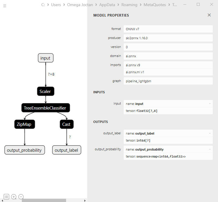
The first output layer is of tensor type with a 1D integer array of unknown size. Resizing this layer to the shape of 1 should work fine. When it comes to the second output layer there is a sequence with a map(resembles a dictionary in Python) with two 1D dimensional arrays of unknown sizes, one for labels and the other for probabilities. That is the way ZipMap puts it, In case you are wondering.

Setting the size of this second output layer using OnnxSetOutputShape for this complex object type is hard and can throw weird errors I wasn't able to figure it out however, resizing it to 1 works fine as it will throw a warning but it still works fine. When you run the ONNX model the proper way. Read more...

   float output_data[];   
   struct Map
     {
      ulong          key[];
      float          value[];
     } output_data_map[];
   
//---

   ArrayResize(output_data, outputs.Size());
    
   if (!OnnxRun(onnx_handle, ONNX_DATA_TYPE_FLOAT, x_float, output_data, output_data_map))
     {
       printf("Failed to get predictions from Onnx err %d",GetLastError());
       return proba;
     }

Inside both Light GBM class and XGBoost we have the following methods:

MQL5 | LightGBM.mqh

class CLightGBM
  {
  
   bool initialized;
   long onnx_handle;
   void PrintTypeInfo(const long num,const string layer,const OnnxTypeInfo& type_info);
   long inputs[], outputs[];
   
   void replace(long &arr[]) { for (uint i=0; i<arr.Size(); i++) if (arr[i] < 0) arr[i] = UNDEFINED_REPLACE; }
   
   bool OnnxLoad(long &handle);
   
public:
                     CLightGBM(void);
                    ~CLightGBM(void);
                     
                     virtual bool Init(const uchar &onnx_buff[], ulong flags=ONNX_DEFAULT); //Initilaized ONNX model from a resource uchar array with default flag
                     virtual bool Init(string onnx_filename, uint flags=ONNX_DEFAULT); //Initializes the ONNX model from a .onnx filename given

                     virtual long predict_bin(const vector &x); //REturns the predictions for the current given matrix | useful in real-time prediction
                     virtual vector predict_proba(const vector &x); //Returns the predictions in probability terms | useful in real-time prediction
                     virtual matrix predict_proba(const matrix &x); //Returns the predicted probability for the whole matrix | useful for testing
                     virtual vector predict_bin(const matrix &x); //gives out the vector for all the predictions | useful for testing
  };

Using LightGBM and XGBoost in Trading

After the model is initialized in the OnInit function.

MQL5 | LightGBM EA.mq5

int OnInit()
  {
   if (!lgbm.Init(lightgbm_onnx))
     return INIT_FAILED;
  }

The loaded ONNX models can be deployed with data collected in the same way as the training data.

void OnTick()
  {

   int size = CopyRates(Symbol(), PERIOD_CURRENT, 1, 1, rates_x); //We copy only one recent-closed bar
   
//---
   
   if (NewBar())
    {
       vector x = {
         rates_x[0].open,
         rates_x[0].high,
         rates_x[0].low,
         rates_x[0].close,
         rates_x[0].close-rates_x[0].open,
         rates_x[0].high-rates_x[0].low,
         rates_x[0].close-rates_x[0].low,
         rates_x[0].close-rates_x[0].high
       };
       
       long signal = lgbm.predict_bin(x);   
       
       Comment("Signal: ",signal);
 }

Let us make a simple trading strategy based on the signals obtained.

   if (NewBar()) //Trade at the opening of a new candle
    {
       vector x = {
         rates_x[0].open,
         rates_x[0].high,
         rates_x[0].low,
         rates_x[0].close,
         rates_x[0].close-rates_x[0].open,
         rates_x[0].high-rates_x[0].low,
         rates_x[0].close-rates_x[0].low,
         rates_x[0].close-rates_x[0].high
       };
       
       
       long signal = lgbm.predict_bin(x);   
       
       Comment("Signal: ",signal);
       
//---
      
      MqlTick ticks;
      SymbolInfoTick(Symbol(), ticks);
      
      if (signal==1) //if the signal is bullish
       {
          if (!PosExists(POSITION_TYPE_BUY)) //There are no buy positions
            m_trade.Buy(lotsize, Symbol(), ticks.ask, ticks.bid-stoploss*Point(), ticks.ask+takeprofit*Point()); //Open a buy trade
       }
      else //Bearish signal
        {
          if (!PosExists(POSITION_TYPE_SELL)) //There are no Sell positions
            m_trade.Sell(lotsize, Symbol(), ticks.bid, ticks.ask+stoploss*Point(), ticks.bid-takeprofit*Point()); //open a sell trade
        }
    }

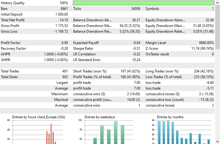
I ran a test on the Strategy-tester, on a 1-hour timeframe on EURUSD from 01.01.2023 to 23.05.2024

LightGBM:

lightgbm report

XGBoost:

xgboost model tester report

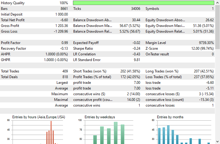
Both models made losses. XGBoost made -8$ fewer losses than LightGBM. They both had a balance chart that looked almost the same.

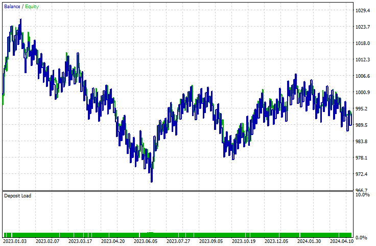
Lightgbm & xgboost strategy tester balance chart

The Strategy Tester report can not tell us if the models are doing a fine job they are trained for which is predicting the next bar movement. As we know a lot of things must be considered to make an Expert Advisor profitable.

To understand how the models were performing lets make a script to collect data the same way we collected the training data, In doing so we make a target variable.

void OnStart()
  {
//---
   if (!lgb.Init(lightgbm_onnx))
     return;
     
//--- custom out-of-sample testing 
   
   int bars = 9000;
   int start = 1000; 
   
   MqlRates rates_x[];
   ArraySetAsSeries(rates_x, true);
   int size = CopyRates(Symbol(), PERIOD_CURRENT, start, bars, rates_x); //We start at the bar 1000 and collect 9000 candles backward
   
   MqlRates rates_y[];
   ArraySetAsSeries(rates_y, true);
   CopyRates(Symbol(), PERIOD_CURRENT, start-1, bars, rates_y); //We do the same thing here but we only collect one bar forward making sure we get the prediction for the next candle
   
//---
   
   vector actual(size), predictions(size);
   for (int i=0; i<size; i++)
     {
       vector x = {
         rates_x[i].open,
         rates_x[i].high,
         rates_x[i].low,
         rates_x[i].close,
         rates_x[i].close-rates_x[i].open,
         rates_x[i].high-rates_x[i].low,
         rates_x[i].close-rates_x[i].low,
         rates_x[i].close-rates_x[i].high
       };
       
       actual[i] = rates_y[i].close > rates_x[i].open ? 1 : 0; //making the target variable
       predictions[i] = (double)lgb.predict_bin(x);
     }
   
   Metrics::classification_report(actual, predictions);
  }

Results | Experts tab:

EG 0 15:18:16.874 LightGBM Performance TestScript (EURUSD,H1) Confusion Matrix

PO 0 15:18:16.874 LightGBM Performance TestScript (EURUSD,H1) [[2857,1503]

CI 0 15:18:16.874 LightGBM Performance TestScript (EURUSD,H1) [926,3714]]

FM 0 15:18:16.874 LightGBM Performance TestScript (EURUSD,H1)

NF 0 15:18:16.874 LightGBM Performance TestScript (EURUSD,H1) Classification Report

HJ 0 15:18:16.874 LightGBM Performance TestScript (EURUSD,H1)

KP 0 15:18:16.874 LightGBM Performance TestScript (EURUSD,H1) [CLS] precision recall specificity f1 score support

QQ 0 15:18:16.874 LightGBM Performance TestScript (EURUSD,H1) [0.0] 0.76 0.66 0.80 0.70 4360

CQ 0 15:18:16.874 LightGBM Performance TestScript (EURUSD,H1) [1.0] 0.71 0.80 0.66 0.75 4640

HS 0 15:18:16.874 LightGBM Performance TestScript (EURUSD,H1)

NK 0 15:18:16.874 LightGBM Performance TestScript (EURUSD,H1) accuracy 0.73 9000

RG 0 15:18:16.874 LightGBM Performance TestScript (EURUSD,H1) average 0.73 0.73 0.73 0.73 9000

LI 0 15:18:16.874 LightGBM Performance TestScript (EURUSD,H1) Weighed avg 0.73 0.73 0.73 0.73 9000

The model was 73% accurate in out-of-sample data. This tells us our model is doing fine despite not being able to produce an upward-heading curve in the strategy tester. This should be a good starting point in making your own profitable Expert Advisors made with GBDTs in MQL5.

Advantages of Gradient-Boosted Decision Trees

1. High Predictive Accuracy

GBDTs often outperform many other machine learning algorithms in terms of predictive accuracy. This is because they combine the strengths of decision trees with gradient boosting, which iteratively improves model performance by focusing on the errors of the previous trees.

2. Robustness to Overfitting

The boosting process involves adding new trees that correct the errors of the existing ensemble, which helps in reducing overfitting. Techniques such as learning rate adjustment, regularization, and early stopping can further enhance this robustness.

3. No Need for Extensive Preprocessing

GBDTs do not require extensive preprocessing steps such as scaling of features, handling of missing values, or encoding of categorical variables, which are typically necessary for other algorithms like linear regression or support vector machines.

4. Flexibility and Customization

GBDTs offer a wide range of hyperparameters that can be tuned to optimize performance for specific tasks. These include the number of trees, learning rate, maximum depth of trees, and the minimum number of samples required to split a node, among others.

5. Handles Complex Relationships

GBDTs can model complex nonlinear relationships between features and the target variable. This makes them suitable for capturing intricate patterns in the data that simpler models might miss.

6. Regularization Techniques

GBDTs include regularization parameters that help to control the complexity of the model and prevent overfitting. Parameters such as max_depth, min_samples_split, and min_samples_leaf play a crucial role in regularization.

7. Scalability

Implementations like XGBoost, LightGBM, and CatBoost are optimized for speed and scalability. They can handle large datasets efficiently and leverage hardware capabilities such as parallel and distributed computing.

As with any machine learning model, these models also have drawbacks that must be acknowledged, not to discourage one from using them but the solidify one's understanding.

Disadvantages of Gradient Boosted Decision Trees

1. Computational Complexity. GBDTs can be computationally expensive to train, especially with a large number of trees and deep trees. In large dataset the training process can consume a significant memory in large and deep datasets

2. Hyperparameter Tuning. Despite being able to work with default parameters for both models discussed, they still have many hyperparameters that need to be carefully tuned to achieve optimal performance. Parameters such as the number of trees, learning rate, maximum depth, and minimum samples per leaf.

As we all know tuning these parameters can be time-consuming and computationally intensive.

3. Still Sensitivity to Noisy Data. Since each tree tries to correct the errors of the previous trees, any noise in the data can be amplified through the boosting process.

4. Often requires Large Datasets. GBDTs often require a large amount of data to achieve good performance. Small datasets might not provide enough information for the boosting process to work effectively.

The Bottom Line

Gradient boosted trees are valuable tools for forex traders, as we have seen them outperform a lot of machine learning model right off the bat. People used to believe complex neural-network based models such as GRU, RNN and LSTM were the go-to models to beat the market but that is no longer the case as gradient boosted trees are growing in popularity in the machine learning community due to their simplicity and their ability to accomplish the predictive task at hand.

Best regards.

Track development of machine learning models and much more discussed in this article series on this GitHub repo.

Python code discussed in this post is linked here.

Attachments Tables:

Expert Advisors | Experts folder:

File name	Description & Usage
LightGBM EA.mq5	An Expert Advisor for testing Light Gradient Boosted Machine (LightGBM)
XGBoost EA.mq5	An expert Advisor for testing Extreme Gradient Boosting (XGBoost)

Libraries | Include folder:

File name	Description & Usage
LightGBM.mqh	A library for loading, initializing and deploying Light Gradient Boosted Machine (LightGBM) ONNX models
XGBoost.mqh	A library for loading, initializing and deploying Extreme Gradient Boosting (XGBoost) ONNX models

Scripts | Scripts folder:

File name	Description & Usage
LightGBM Performance TestScript.mq5	A script for testing LightGBM model in real time

Files | Files folder:

File name	Description & Usage
EURUSD.PERIOD_H1.csv	A csv file containing the training dataset
lightgbm.eurusd.h1.onnx xgboost.eurusd.h1.onnx	LightGBM and XGBoost models in ONNX format

Python code:

File name	Description & Usage
lightgbm-xgboost.ipynb	Jupyter notebook containing all the python code discussed in this post.

Sources and References:

Can one do better than XGBoost? - Mateusz Susik (https://www.youtube.com/watch?v=5CWwwtEM2TA).
Unlocking the Power of Gradient-Boosted Trees (using LightGBM) | PyData London 2022(https://www.youtube.com/watch?v=qGsHlvE8KZM).
LightGBM documentation: (https://lightgbm.readthedocs.io/en/latest/Parameters.html).
XGBoost documentation (https://xgboost.readthedocs.io/en/stable/tutorials/model.html).

Attached files |

Download ZIP

Code_b_Files.zip (173.73 KB)

Warning: All rights to these materials are reserved by MetaQuotes Ltd. Copying or reprinting of these materials in whole or in part is prohibited.

What are Gradient Boosted Trees?

Gradient Boosted Decision Trees (LighGBM & XGBoost) Vs Other Classifiers

What is Extreme Gradient Boosting (XGBoost)?

How does XGBoost Work?

Implementing XGBoost in Python

What is Light Gradient Boosting Machine (LightGBM)?

Light GBM Improvements

How does LightGBM Work?

The differences between XGBoost and Light GBM

Implementing Light GBM in Python

Saving XGBoost and LightGBM to ONNX.

Loading ONNX model in MQL5

Using LightGBM and XGBoost in Trading

Advantages of Gradient-Boosted Decision Trees

Disadvantages of Gradient Boosted Decision Trees

The Bottom Line

Other articles by this author