Data Science and ML (Part 34): Time series decomposition, Breaking the stock market down to the core

Introduction

Time series data forecasting has never been easy. Patterns are often hidden and filled with noise and uncertainties, charts are often misleading since they contain an overview of the market performance which isn't intended to give you in-depth insights on what's happening.

In statistical forecasting and machine learning, what we are trying to do is to break down the time series data which happens to be price values in the market (Open, High, Low, and Close values), into several components that could be more insightful than a single time series array.

In this article, we are going to look at the statistical technique known as seasonal decomposition. We aim to use it to dissect the stock markets to detect the trends, seasonal patterns and much more.

What is Seasonal Decomposition

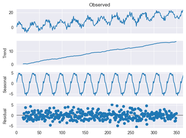
Seasonal decomposition is a statistical technique used to break downtime series data into several components; Trend, Seasonality, and Residual. These components can be explained as follows.

Trend

The trend component of the time series data refers to the long-term changes or patterns that are observed over time.

It represents the general direction in which the data is moving. For example, if the data is increasing over time, the trend component will be upward-sloping, and if the data is decreasing over time, the trend component will be downward-sloping.

This is familiar to almost all traders, the trend is the easiest thing to spot in the market by just looking at the chart.

Seasonality

The seasonal component of a time series data refers to the cynical patterns that are observed within a given period of time. For example, if we are analyzing monthly sales data for a retailer who specialized in decoration and gifts, the seasonal component would capture the fact that sales tend to peak in December due to Christmas shopping, sales flattens once the holiday season is over, in months January, February, etc.

Residual

The residual component of a time series data represents the random variation that is left over after the trend and seasonal components have been accounted for. It represents the noise or error in the data that cannot be explained by the trend or seasonal patterns.

To understand this further, look at the image below.

Why do we do Seasonal Decomposition?

Before we go into mathematical details and implement seasonal decomposition in MQL5, Let's first understand the reasons to why we perform seasonal composition in time series data.

1. To detect underlying patterns and trends in the data
   
   Seasonal decomposition can help us to identify trends and patterns in the data that might not be immediately apparent when examining the raw data, by breaking down the data into its constituent components (trend, seasonal, and residual), we gain a better understanding of how these components contribute to the overall behavior of the data.
   
   
2. To remove the effects of seasonality
   
   Seasonal decomposition can be used to remove the effects of seasonality from the data, allowing us to focus on the underlying trend or the opposite when we are eager to work with seasonal patterns only for example: When working with weather data that exhibit strong seasonal patterns.
   
   
3. To make accurate predictions
   
   When you have data broken down into components, it helps filter the unnecessary information which could be less required depending on a problem, for example, when trying to predict the trend, it is wiser to have the trend information only instead of the seasonal data.
   
   
4. To compare trends across different periods of time or regions
   
   Seasonal decomposition can be used to compare trends across different time-periods or regions, providing insights into how different factors may be affecting the data. For example, if we are comparing retail sales data across different regions, seasonal decomposition can help us to identify regional differences in seasonal patterns and adjust our analyses accordingly.

Implementing Seasonal Decomposition in MQL5

To implement this analytical algorithm, let's first generate some simple random data with trend features, seasonal patters, and some noise, this is something that can be seen in real-life data scenarios, especially in forex and stock markets where data isn't straightforward and clean.

We are going to use Python programming language for the task.

File: seasonal_decomposition_visualization.ipynb

import pandas as pd
import numpy as np
import seaborn as sns
import matplotlib.pyplot as plt
import os

sns.set_style("darkgrid")

# Create synthetic time-series data
np.random.seed(42)
time = np.arange(0, 365)  # 1 year (daily data)
trend = 0.05 * time  # Linear upward trend
seasonality = 5 * np.sin(2 * np.pi * time / 30)  # 30-day periodic seasonality
noise = np.random.normal(scale=2, size=len(time))  # Random noise

# Combine components to form the time-series
time_series = trend + seasonality + noise

# Plot the original time-series
plt.figure(figsize=(10, 4))
plt.plot(time, time_series, label="Original Time-Series", color="blue")
plt.xlabel("Time (Days)")
plt.ylabel("Value")
plt.title("Synthetic Time-Series with Trend and Seasonality")
plt.legend()
plt.show()

Outcome

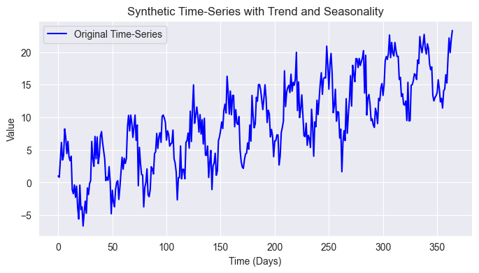
We know that the stock market is more complex than that but, given this simple data, lets attempt to uncover the 30 days seasonality patterns that we added to the time series, the overall trend, and filter some noise from the data.

Trend Extraction

To extract the trend features we can use the moving average (MA) as it smooths a time series by averaging values over a fixed window. This helps filter out short-term fluctuations and highlight the underlying trend.

In additive decomposition, the trend is estimated using a moving average over a window equal to the seasonal period p.

Where:

 = Trend component at time t.

 = Window size or seasonal period.

 = Half of the seasonal period.

 = Observed time series values.

For multiplicative decomposition, we take the geometric mean instead.

Where:

 = Product operator, where instead of summing, we multiply all the values within the window because multiplicative decomposition assumes that seasonal effects scale the data rather than adding to it.

This might seem like complex maths, but it can be broken down into a few lines of MQL5 code.

vector moving_average(const vector &v, uint k, ENUM_VECTOR_CONVOLVE mode=VECTOR_CONVOLVE_VALID)
 {
   vector kernel = vector::Ones(k) /  k;
   vector ma = v.Convolve(kernel, mode);
    
   return ma;  
 }

We calculate the moving average based on the convolve method because it is flexible, efficient, and handles missing values at the edges of the array, unlike calculating the moving average using the rolling window approach.

We can finalize the formula as follows.

//--- compute the trend

   int n = (int)timeseries.Size();  
   res.trend = moving_average(timeseries, period);
   
   // We align trend array with the original series length
   
   int pad = (int)MathFloor((n - res.trend.Size()) / 2.0);
   int pad_array[] = {pad, n-(int)res.trend.Size()-pad};
   
   res.trend = Pad(res.trend, pad_array, edge);

Seasonal Component Extraction

Seasonal component extraction refers to isolating the repeated patterns in a time series that occur at a given interval for example; daily, monthly, yearly, etc.

This component is computed after removing the trend from the original time series data, it can be extracted differently depending on whether the model is additive or multiplicative.

Additive model

After estimating the trend  , the de-trended series is computed as follows.

Where:

 = a de-trended value at time t.

 =  time series value at time t.

 = trend component at time t.

To compute the seasonal component, we take the average of the de-trended values over all complete cycles of the seasonal period p.

Where:

 = number of full seasonal cycles in the dataset.

 = the seasonal period (e.g. 30 for daily data in a monthly cycle).

 = Extracted seasonal component.

Multiplicative model

When it comes to the multiplicative model, we divide instead of subtracting to detrend a time series.

The seasonal component is extracted by taking the geometric mean instead of the arithmetic mean.

This helps to prevent bias due to the multiplicative nature of the model.

We can implement this function in MQL5 as follows.

//--- compute the seasonal component
   
   if (model == multiplicative)
     {
       for (ulong i=0; i<timeseries.Size(); i++)
         if (timeseries[i]<=0)
            {
               printf("Error, Multiplicative seasonality is not appropriate for zero and negative values");
               return res;
            }
     }
   
   vector detrended = {};
   vector seasonal = {};
   
   switch(model)
     {
      case  additive:
        {
          detrended = timeseries - res.trend;
          seasonal = vector::Zeros(period);
         
          for (uint i = 0; i < period; i++)
            seasonal[i] = SliceStep(detrended, i, period).Mean(); //Arithmetic mean over cycles
        }    
        break;
      case  multiplicative:
        {
          detrended = timeseries / res.trend;
          seasonal = vector::Zeros(period);
         
          for (uint i = 0; i < period; i++)
            seasonal[i] = MathExp(MathLog(SliceStep(detrended, i, period)).Mean()); //Geometric mean
        }    
        break;
      default:
        printf("Unknown model for seasonal component calculations");
        break;
     }

    
    vector seasonal_repeated = Tile(seasonal, (int)MathFloor(n/period)+1);
    res.seasonal = Slice(seasonal_repeated, 0, n);

The Pad function, adds padding (extra values) around a vector, similarly to Numpy.pad in this scenario it helps to ensure the moving average values are centered.

Due to the presence of a Logarithmic transformation function MathLog which can not be used for zero and negative values, the multiplicative model should be restricted to only positive time series, this condition had to be checked and reinforced.

   if (model == multiplicative)
     {
       for (ulong i=0; i<timeseries.Size(); i++)
         if (timeseries[i]<=0)
            {
               printf("Error, Multiplicative seasonality is not appropriate for zero and negative values");
               return res;
            }
     }

The Tile function constructs a large vector by repeating the seasonal vector several times. This process is crucial for capturing the repeated seasonal patterns in a time series.

Residual Calculation

Finally, we calculate the residuals by subtracting the trend and seasonality.

For additive model:

For multiplicative model:

Where:

 = original time series value at time t.

 = trend value at time t.

 = seasonal value at time t.

Putting it All in One Function

Similarly to the seasonal_decompose function which I took inspiration from, I had to wrap all the calculations in one function named seasonal_decompose which returns a structure containing trend, seasonal, and residual vectors.

enum seasonal_model
 {
   additive,
   multiplicative
 };

struct seasonal_decompose_results
 {
   vector trend;
   vector seasonal;
   vector residuals;
 };
 
seasonal_decompose_results seasonal_decompose(const vector &timeseries, uint period, seasonal_model model=additive)
 {
   seasonal_decompose_results res;
   
   if (timeseries.Size() < period)
    {
      printf("%s Error: Time series length is smaller than the period. Cannot compute seasonal decomposition.",__FUNCTION__);
      return res;
    }
   
//--- compute the trend

   int n = (int)timeseries.Size();  
   res.trend = moving_average(timeseries, period);
   
   // We align trend array with the original series length
   
   int pad = (int)MathFloor((n - res.trend.Size()) / 2.0);
   int pad_array[] = {pad, n-(int)res.trend.Size()-pad};
   
   res.trend = Pad(res.trend, pad_array, edge);

//--- compute the seasonal component
   
   if (model == multiplicative)
     {
       for (ulong i=0; i<timeseries.Size(); i++)
         if (timeseries[i]<=0)
            {
               printf("Error, Multiplicative seasonality is not appropriate for zero and negative values");
               return res;
            }
     }
   
   vector detrended = {};
   vector seasonal = {};
   
   switch(model)
     {
      case  additive:
        {
          detrended = timeseries - res.trend;
          seasonal = vector::Zeros(period);
         
          for (uint i = 0; i < period; i++)
            seasonal[i] = SliceStep(detrended, i, period).Mean(); //Arithmetic mean over cycles
        }    
        break;
      case  multiplicative:
        {
          detrended = timeseries / res.trend;
          seasonal = vector::Zeros(period);
         
          for (uint i = 0; i < period; i++)
            seasonal[i] = MathExp(MathLog(SliceStep(detrended, i, period)).Mean()); //Geometric mean
        }    
        break;
      default:
        printf("Unknown model for seasonal component calculations");
        break;
     }


    
    vector seasonal_repeated = Tile(seasonal, (int)MathFloor(n/period)+1);
    res.seasonal = Slice(seasonal_repeated, 0, n);

//--- Compute Residuals

    if (model == additive)
        res.residuals = timeseries - res.trend - res.seasonal;
    else  // Multiplicative
        res.residuals = timeseries / (res.trend * res.seasonal);
        
   return res;
 }

We can finally test this function.

I had to generate positive values too and save them in a CSV file for testing seasonal decomposition using the multiplicative model.

File: seasonal_decomposition_visualization.ipynb

# Create synthetic time-series data
np.random.seed(42)
time = np.arange(0, 365)  # 1 year (daily data)
trend = 0.05 * time  # Linear upward trend
seasonality = 5 * np.sin(2 * np.pi * time / 30)  # 30-day periodic seasonality
noise = np.random.normal(scale=2, size=len(time))  # Random noise

# Combine components to form the time-series
time_series = trend + seasonality + noise

# Fix for multiplicative decomposition: Shift the series to make all values positive
min_value = np.min(time_series)
if min_value <= 0:
    shift_value = abs(min_value) + 1  # Ensure strictly positive values
    time_series_shifted = time_series + shift_value
else:
    time_series_shifted = time_series

ts_pos_df = pd.DataFrame({
    "timeseries": time_series_shifted
})

ts_pos_df.to_csv(os.path.join(files_path,"pos_ts_df.csv"), index=False)

Inside our MQL5 script, we load both time series datasets using the dataframe library we discussed in this article, After loading the data we run the seasonal decompose algorithms.

File: seasonal_decompose test.mq5

#include <MALE5\Stats Models\Tsa\Seasonal Decompose.mqh>
#include <MALE5\pandas.mqh>
//+------------------------------------------------------------------+
//| Script program start function                                    |
//+------------------------------------------------------------------+
void OnStart()
  {
//--- Additive model
   
   CDataFrame df;
   df.FromCSV("ts_df.csv");
   
   vector time_series = df["timeseries"];
   
//---
    
    seasonal_decompose_results res_ad = seasonal_decompose(time_series, 30, additive);
    
    df.Insert("original", time_series);
    df.Insert("trend",res_ad.trend);
    df.Insert("seasonal",res_ad.seasonal);
    df.Insert("residuals",res_ad.residuals);
    
    df.ToCSV("seasonal_decomposed_additive.csv");

//--- Multiplicative model

   CDataFrame pos_df;
   pos_df.FromCSV("pos_ts_df.csv");
   
   time_series = pos_df["timeseries"];
   
//---
    
    seasonal_decompose_results res_mp = seasonal_decompose(time_series, 30, multiplicative);
    
    pos_df.Insert("original", time_series);
    pos_df.Insert("trend",res_mp.trend);
    pos_df.Insert("seasonal",res_mp.seasonal);
    pos_df.Insert("residuals",res_mp.residuals);
    
    pos_df.ToCSV("seasonal_decomposed_multiplicative.csv");
  }

I had to save the outcome back to new CSV files for visualization using Python.

Seasonal decomposition using additive model outcome plot

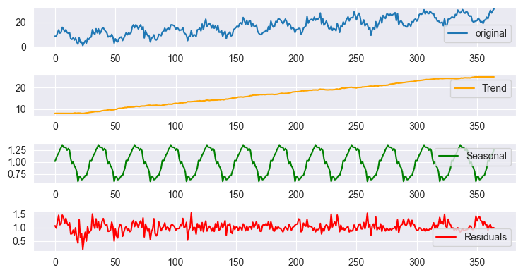
Seasonal decomposition using multiplicative model outcome plot

The plots look almost similar when plotted due to the scale but the outcomes differs when you look at the data. This is the same outcome you would get using tsa.seasonal.seasonal_decompose provided by stats models in Python.

Now that we have the seasonal decompose function, let's use it to analyze the stock markets.

Observing Patterns in the Stock Market

When analyzing the stock market, identifying the trend is often straightforward especially for well-established and fundamentally strong companies. Many large, financially stable corporations tend to follow an upward trajectory over time due to consistent growth, innovation, and market demand.

However, detecting seasonal patterns in stock prices can be much more challenging. Unlike trends, seasonality refers to recurring price movements at fixed intervals which may not always be obvious, these patterns can occur at different timeframes.

Intraday seasonality

Certain hours in a trading day may exhibit repetitive price behavior (e.g., increased volatility at the market openingor closing).

Monthly or quarterly seasonality

Stock prices may follow cycles based on earnings reports, economic conditions, or investor sentiment.

Long-term seasonality

Some stocks show repetitive trends over the years due to economic cycles or company-specific factors.

Case Study, The Apple (AAPL) Stock

Using Apple’s stock as an example, we can hypothesize that seasonal patterns emerge every 22 trading days, which corresponds to roughly one trading month in a yearly dataset. This assumption is based on the fact that there are approximately 22 trading days per month (excluding weekends and holidays).

By applying seasonal decomposition techniques, we can analyze whether Apple's stock exhibits recurring price movements every 22 days. If a strong seasonality component is present, it suggests that price fluctuations may follow predictable cycles, which can be useful for traders and analysts, however, if no significant seasonality is detected, price movements may be largely driven by external factors, noise, or a dominant trend.

Let's collect the daily closing prices for 1000 bars and perform multiplicative seasonal decomposition on a period of 22 days.

#include <MALE5\Stats Models\Tsa\Seasonal Decompose.mqh>
#include <MALE5\pandas.mqh>

input uint bars_total = 1000;
input uint period_ = 22;
//+------------------------------------------------------------------+
//| Script program start function                                    |
//+------------------------------------------------------------------+
void OnStart()
  {
//---
   
    vector close, time;
    close.CopyRates(Symbol(), PERIOD_D1, COPY_RATES_CLOSE, 1, bars_total); //closing prices
    time.CopyRates(Symbol(), PERIOD_D1, COPY_RATES_TIME, 1, bars_total); //time
   
    seasonal_decompose_results res_ad = seasonal_decompose(close, period_, multiplicative);
    
    CDataFrame df; //A dataframe object for storing the seasonal decomposition outcome
    
    df.Insert("time", time);
    df.Insert("close", close);
    df.Insert("trend",res_ad.trend);
    df.Insert("seasonal",res_ad.seasonal);
    df.Insert("residuals",res_ad.residuals);
    
    df.ToCSV(StringFormat("%s.%s.period=%d.seasonal_dec.csv",Symbol(), EnumToString(PERIOD_D1), period_));
  }

The outcome was then visualized in a Jupyter notebook named stock_market seasonal dec.ipynb below is the outcome.

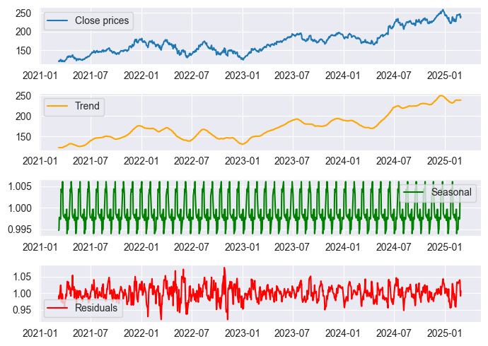
Okay, we can see some seasonal patterns in the above plot but, we cannot be 100% sure of the seasonal patterns because there are always some errors associated, the challenge would be to interpret the error values and make your analysis accordingly.

Based on the residuals plot we can see that there are spikes in residual values in the years 2020 to 2022, we all know this was the period when there was a global pandemic, so maybe the seasonal patterns were disrupted and inconsistent indicating we can't trust the seasonal patterns we see in that period.

Rule of thumb.

Good decomposition:  Residuals should look like random noise (white noise).

Bad decomposition: Residuals still show visible structure (trends or seasonal effects that weren’t removed).

We can use different mathematical techniques to visualize the residuals such as;

The distribution plot

We have a normally distributed residuals plot, this could be a good sign that there could be some monthly patterns in the Apple Stock.

The Mean and Standard deviation

In the additive model, the residuals mean should be close to 0 meaning the most variations are explained by the trend and seasonality.

In multiplicative model, the residual mean is ideally close to 1, meaning the original series is well explained by the trend and seasonality.

The standard deviation value needs to be small

print("Residual Mean:", residuals.mean())  # Should be close to 0
print("Residual Std Dev:", residuals.std())  # Should be small

Outputs

Residual Mean: 1.0002367590572043
Residual Std Dev: 0.021749969975933727

Finally, we can put it all inside an indicator.

#property indicator_separate_window
#property indicator_buffers 2
#property indicator_plots 1

#property indicator_color1 clrDodgerBlue
#property indicator_style1 STYLE_SOLID
#property indicator_type1 DRAW_LINE
#property indicator_width1 2

//+------------------------------------------------------------------+

double trend_buff[];
double seasonal_buff[];

#include <MALE5\Stats Models\Tsa\Seasonal Decompose.mqh>
#include <MALE5\pandas.mqh>

input uint bars_total = 10000;
input uint period_ = 22;
input ENUM_COPY_RATES price = COPY_RATES_CLOSE;

//+------------------------------------------------------------------+
//| Custom indicator initialization function                         |
//+------------------------------------------------------------------+
int OnInit()
  {
//--- indicator buffers mapping
   
   SetIndexBuffer(0, seasonal_buff, INDICATOR_DATA);
   SetIndexBuffer(1, trend_buff, INDICATOR_CALCULATIONS);
   
//---
   
   IndicatorSetString(INDICATOR_SHORTNAME, "Seasonal decomposition("+string(period_)+")");
   PlotIndexSetString(1, PLOT_LABEL, "seasonal ("+string(period_)+")");
   
   PlotIndexSetDouble(0, PLOT_EMPTY_VALUE, 0.0);
   
   ArrayInitialize(seasonal_buff, EMPTY_VALUE);
   ArrayInitialize(trend_buff, EMPTY_VALUE);
    
   return(INIT_SUCCEEDED);
  }

//+------------------------------------------------------------------+
//| Custom indicator iteration function                              |
//+------------------------------------------------------------------+
int OnCalculate(const int rates_total,
                const int prev_calculated,
                const datetime &time[],
                const double &open[],
                const double &high[],
                const double &low[],
                const double &close[],
                const long &tick_volume[],
                const long &volume[],
                const int &spread[])
  {
//---
    
    if (prev_calculated==rates_total) //not on a new bar, calculate the indicator on the opening of a new bar  
      return rates_total;
    
    ArrayInitialize(seasonal_buff, EMPTY_VALUE);
    ArrayInitialize(trend_buff, EMPTY_VALUE);

//---

    Comment("rates total: ",rates_total," bars total: ",bars_total);
    
    //if (rates_total<(int)bars_total)
    //  return rates_total;
          
    vector close_v;
    close_v.CopyRates(Symbol(), Period(), price, 0, bars_total); //closing prices
      
    seasonal_decompose_results res = seasonal_decompose(close_v, period_, multiplicative);
    
    for (int i=MathAbs(rates_total-(int)bars_total), count=0; i<rates_total; i++, count++) //calculate only the chosen number of bars
      {
         trend_buff[i] = res.trend[count];
         seasonal_buff[i] = res.seasonal[count];
      }
    
//--- return value of prev_calculated for next call
   return(rates_total);
  }

Due to the nature of seasonal decomposition calculation, it can be computationally expensive to calculate when we use all the rates available in the chart to compute as soon as new rates arrive on the chart, we have to restrict the number of bars to use for calculation and plotting.

I had to create two separate indicators one for plotting seasonal patterns and the other for plotting the residuals using the same logic.

Below are the indicator plots on the Apple symbol. 

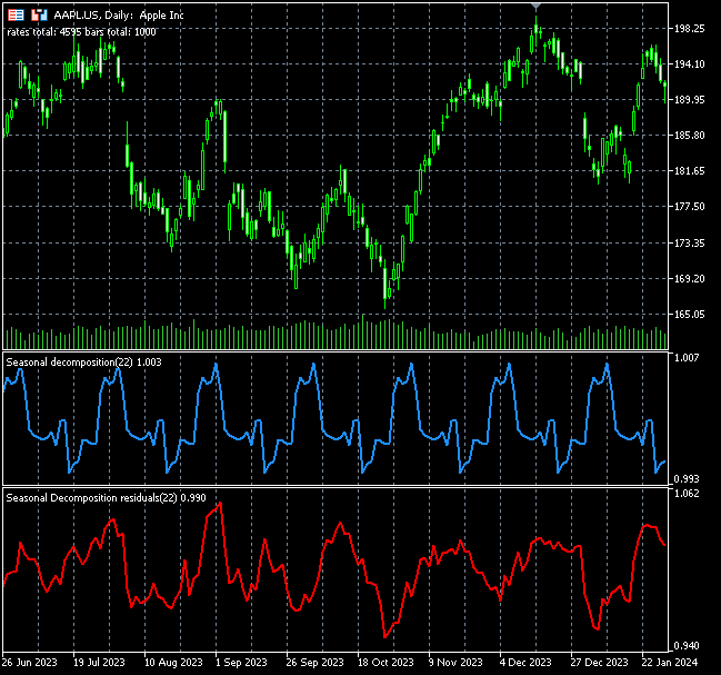
The indicator's seasonal patterns can also be interpreted as trading signals or oversold and overbought conditions as it can be seen on the chart above, right now, it's difficult to tell as I am yet to explore it on a trading side. I encourage you to do so as a homework.

Final Thoughts

Seasonal decomposition is a useful technique to have in your algorithmic trading toolbox, some data scientists use it to create new features based on the time series data they have at hand while others use it to analyze the nature of the data and then decide the right machine learning techniques to use for the particular problem, this now raises an important question of when to use seasonal decomposition?. 

Some data scientists start by performing seasonal decomposition to separate the time series into its underlying components: trend, seasonality, and residuals. If there is a clear seasonal pattern in the data, then seasonal exponential smoothing (also known as the seasonal Holt-Winters method) is deployed to attempt to forecast the data, however, if there is not a clear seasonal pattern, or if the seasonal pattern is weak or irregular, then ARIMA models and other standard machine learning models are deployed to attempt to unveil the patterns in the time series data and make predictions.

Attachments table

Filename & Path	Description & Usage
Include\pandas.mqh	Consists of the Dataframe class for data storage and manipulation in Pandas-like format.
Include\Seasonal Decompose.mqh	Contains all the functions and lines of code that make seasonal decomposition possible in MQL5.
Indicators\Seasonal Decomposition.mq5	This indicator plots the seasonal component.
Indicators\Seasonal Decomposition residuals.mq5	This indicator plots the residual component.
Scripts\seasonal_decompose test.mq5	A  simple script used to implement and debug the seasonal decompose function and its constituents.
Scripts\stock market seasonal dec.mq5	A script for analyzing the closing price of a symbol and saving the outcome to a CSV file for analytical purposes
Python\seasonal_decomposition_visualization.ipynb	Jupyter notebook for visualizing seasonal decomposition outcomes in CSV files.
Python\stock_market seasonal dec.ipynb	Jupyter notebook for visualizing the seasonal decomposition results of a stock.
Files\*.csv	CSV files containing seasonal decomposition outcomes and data from both Python code and MQL5.