Build Self Optimizing Expert Advisors With MQL5 And Python (Part II): Tuning Deep Neural Networks

Introduction

Members of our community are keen to integrate AI into their trading strategies, which requires tuning AI models for specific markets. Each AI model has adjustable parameters that significantly influence its performance; optimal settings for one market may not work for another. This article will show how to customize AI models to outperform default settings using optimization algorithms, specifically the Nelder-Mead algorithm. We'll apply this algorithm to fine-tune a deep neural network using data from the MetaTrader5 terminal and then export the optimized model in ONNX format for use in an Expert Advisor. For those unfamiliar with these concepts, we will provide detailed explanations throughout the article.

Nelder-Mead Optimization Algorithm

The Nelder-Mead algorithm is a popular choice for noisy, non-differentiable, and non-linear multimodal optimization problems. Named after its inventors John Nelder and Roger Mead, the algorithm was introduced in their 1965 paper titled "A Simplex Method for Function Minimization." It can be used for both univariate and multivariate optimization problems.

The Nelder-Mead algorithm does not rely on derivative information; instead, it is a pattern search optimization algorithm. It requires the user to provide a starting point. Depending on the chosen starting point, the algorithm might get stuck in a deceptive local optimum. Therefore, it can be beneficial to perform the optimization multiple times with different starting points to improve the chances of finding a global optimum.

The algorithm works by using a geometric shape called a simplex. The simplex has one vertex for each input variable plus one additional vertex. The points (vertices) of the simplex are evaluated, and simple rules are used to move the points based on their evaluations. The algorithm has certain stopping conditions, such as reaching the maximum number of iterations or achieving a minimal change in evaluation values. If no improvements are made or if the allowed number of iterations is exceeded, the optimization procedure stops.

Fig 1: Roger Mead

Fig 2: John Nelder

Let’s Get Started

We start by fetching the data we need from our MetaTrader 5 terminal. First, we open up our MetaTrader 5 Terminal and click the Symbol icon in the context menu. From there, we select bars and search for the symbol you'd like to use. Once you've requested the data, simply click export and the data will be available for you in CSV format.

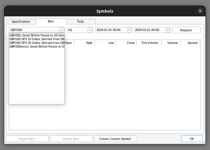
Fig 3: Search for the data you need

Since our data is ready, we can start by importing the libraries we need.

#import libraries we need
import pandas as pd
import numpy as np
from numpy.random import randn,rand
import seaborn as sns

Then we read in the data we prepared.

#Read in our market data
brent = pd.read_csv("/home/volatily/market_data/Market Data UK Brent Oil.csv", sep="\t")

We need to label our data.

#Preparing to label the data
look_ahead = 20

#Defining the target
brent["Target"] = brent["Close"].shift(-look_ahead)

#Drop missing values
brent.dropna(inplace=True)

Let us import the libraries we need for optimization.

#In this article we will cover some techniques for hyper-parameter tuning 
from scipy.optimize import minimize
from sklearn.neural_network import MLPRegressor
from sklearn.model_selection import TimeSeriesSplit
from sklearn.metrics import root_mean_squared_error
import time

We shall now create our time series cross validation object.

#Define the time series split parameters
splits = 5
gap = look_ahead

#Create the time series split object
tscv = TimeSeriesSplit(n_splits=splits,gap=gap)

#Create a dataframe to store our accuracy 
current_error_rate = pd.DataFrame(index = np.arange(0,splits),columns=["Current Error"])

Let us define the predictors and targets for our model.

#Define the predictors and the target
predictors = ["Open","High","Low","Close"]
target = "Target"

We now define the function we aim to minimize: the cross-validation error of the model. Please note that this is for demonstration purposes only. Ideally, we would partition the dataset in half, performing optimization on one half and measuring accuracy on the other half. However, for this demonstration, we are optimizing the model and measuring its accuracy using the same dataset.

#Define the objective function
def objective(x):
    #The parameter x represents a new value for our neural network's settings
    #In order to find optimal settings, we will perform 10 fold cross validation using the new setting
    #And return the average RMSE from all 10 tests
    #We will first turn the model's Alpha parameter, which controls the amount of L2 regularization
    model = MLPRegressor(hidden_layer_sizes=(5,2),alpha=x[0],early_stopping=True,shuffle=False,learning_rate_init=x[1],tol=x[2])
    #Now we will cross validate the model
    for i,(train,test) in enumerate(tscv.split(brent)):
        #The data
        X_train = brent.loc[train[0]:train[-1],predictors]
        y_train = brent.loc[train[0]:train[-1],target]
        X_test  = brent.loc[test[0]:test[-1],predictors]
        y_test  = brent.loc[test[0]:test[-1],target]
        #Train the model
        model.fit(X_train,y_train)
        #Measure the RMSE
        current_error_rate.iloc[i,0] = root_mean_squared_error(y_test,model.predict(X_test))
    #Return the Mean CV RMSE
    return(current_error_rate.iloc[:,0].mean())

Recall that the Nelder-Mead algorithm requires an initial starting point. To find a good starting point, we will perform a line search over the parameters in question. We will use a for loop to measure our accuracy with parameters set to 0.1, then 0.01, and so on. This will help us identify a potentially good starting point for the algorithm.

#Let us measure how much time this takes.
start = time.time()

#Create a dataframe to measure the error rates
starting_point_error = pd.DataFrame(index=np.arange(0,21),columns=["Average CV RMSE"])
starting_point_error["Iteration"] = np.arange(0,21)

#Let us first find a good starting point for our optimization algorithm
for i in np.arange(0,21):
    #Set a new starting point
    new_starting_point = (10.0 ** -i)
    #Store error rates
    starting_point_error.iloc[i,0] = objective([new_starting_point,new_starting_point,new_starting_point]) 

#Record the time stamp at the end
stop = time.time()

#Report the amount of time taken
print(f"Completed in {stop - start} seconds")

Completed in 312.29402351379395 seconds

Let us now observe our error levels.

Average CV RMSE	Iteration
0.91546	0
0.267167	1
14.846035	2
15.763264	3
56.820397	4
75.202923	5
72.562681	6
64.33746	7
88.980977	8
83.791834	9
82.871215	10
88.031151	11
65.532539	12
78.177191	13
85.063947	14
88.631589	15
74.369735	16
86.133656	17
90.482654	18
102.803612	19
74.636781	20

As we can see, it appears that we passed over an optimal region between iteration 0 and 2. From then on, our error kept increasing. We can observe the same information visually.

sns.lineplot(data=starting_point_error,x="Iteration",y="Average CV RMSE")

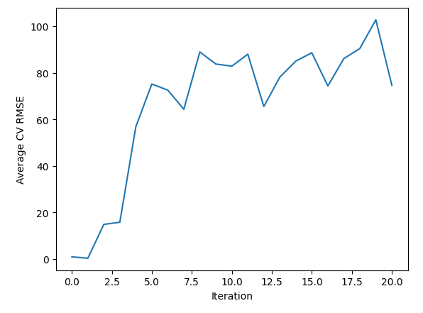
Fig 4: Visualizing the results of our line search

Since we have gained an idea of what a good starting point may be, let us define a function to give us random points within the range we believe the optima may be in.

pt = abs(((10 ** -1) + rand(3) * ((10 ** 0) - (10 ** -1))))
pt

array([0.75747551, 0.34066536, 0.26214705])

Notice that we are fetching an array of 3 random values because we are optimizing 3 different parameters on our neural network. Let us now perform the hyperparameter tuning.

start = time.time()
result = minimize(objective,pt,method="nelder-mead")
stop = time.time()
print(f"Task completed in {stop - start} seconds")

Task completed in 1332.9911317825317 seconds

Let us interpret the result of the optimization

result

message: Maximum number of function evaluations has been exceeded.
       success: False
        status: 1
           fun: 0.12022686955703668
             x: [ 7.575e-01  3.577e-01  2.621e-01]
           nit: 225
          nfev: 600
 final_simplex: (array([[ 7.575e-01,  3.577e-01,  2.621e-01],
                       [ 7.575e-01,  3.577e-01,  2.621e-01],
                       [ 7.575e-01,  3.577e-01,  2.621e-01],
                       [ 7.575e-01,  3.577e-01,  2.621e-01]]), array([ 1.202e-01,  2.393e-01,  2.625e-01,  8.978e-01])

First, observe the user-friendly message displayed at the top. The message indicates that the algorithm has exceeded the maximum number of function evaluations. Recall the conditions we specified earlier regarding the scenarios that would cause the optimization to halt. While we can try increasing the number of allowed iterations, it does not guarantee better performance.

We can see the key 'fun,' which indicates the optimal output the algorithm achieved from the function. Following that is the key 'x,' which shows the values of x that resulted in the optimal output.

We can also observe the 'nit' key, which tells us the number of iterations the function performed. Lastly, the 'nfev' key indicates the number of times the algorithm called the objective function to evaluate its output. Recall that our objective function performed 5-fold cross-validation and returned the average error rate. This means that each time we call the function once, we fit our neural network 5 times. Therefore, 600 function evaluations mean we fit our neural network 3000 times!

Let us now compare the default model and the customized model we built.

#Let us compare our customised model and the defualt model
custom_model = MLPRegressor(hidden_layer_sizes=(5,2),alpha=result.x[0],early_stopping=True,shuffle=False,learning_rate_init=result.x[1],tol=result.x[2])

#Default model
default_model = MLPRegressor(hidden_layer_sizes=(5,2))

We will prepare the time series split object.

#Define the time series split parameters
splits = 10
gap = look_ahead

#Create the time series split object
tscv = TimeSeriesSplit(n_splits=splits,gap=gap)

#Create a dataframe to store our accuracy 
model_error_rate = pd.DataFrame(index = np.arange(0,splits),columns=["Default Model","Custom Model"])

We shall now cross validate each model.

#Now we will cross validate the model
for i,(train,test) in enumerate(tscv.split(brent)):
    #The data
    X_train = brent.loc[train[0]:train[-1],predictors]
    y_train = brent.loc[train[0]:train[-1],target]
    X_test  = brent.loc[test[0]:test[-1],predictors]
    y_test  = brent.loc[test[0]:test[-1],target]
    #Our model
    model = MLPRegressor(hidden_layer_sizes=(5,2),alpha=result.x[0],early_stopping=True,shuffle=False,learning_rate_init=result.x[1],tol=result.x[2])
    #Train the model
    model.fit(X_train,y_train)
    #Measure the RMSE
    model_error_rate.iloc[i,1] = root_mean_squared_error(y_test,model.predict(X_test))

Let us observe our error metrics.

model_error_rate

Default Model	Customized Model
0.153904	0.550214
0.113818	0.501043
82.188345	0.52897
0.114108	0.117466
0.114718	0.112892
77.508403	0.258558
0.109191	0.304262
0.142143	0.363774
0.163161	0.153202
0.120068	2.20102

Let us also visualize the results.

model_error_rate["Default Model"].plot(legend=True)
model_error_rate["Custom Model"].plot(legend=True)

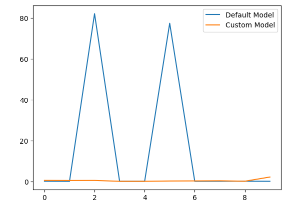
Fig 5: Visualizing the performance of our customized model

As we can observe, the customized model outperformed the default model. However, our test would have been more convincing if we had used separate datasets for training the models and evaluating their accuracy. Using the same dataset for both purposes is not the ideal procedure.

Next, we will prepare to convert our deep neural network into its ONNX representation. ONNX, which stands for Open Neural Network Exchange, is a standardized format that allows AI models trained in any compliant framework to be used in different programs. For example, ONNX allows us to train an AI model in Python and then use it in MQL5 or even a Java program (provided the Java API supports ONNX).

First, we import the libraries we need.

#Now we will prepare to export our neural network into ONNX format
from skl2onnx.common.data_types import FloatTensorType
from skl2onnx import convert_sklearn
import onnxruntime as ort
import netron

Let us define the input shape for our model, remember our model takes 4 inputs.

#Define the input types
initial_type = [("float_input",FloatTensorType([1,4]))]

Fitting our customized model.

#Fit our custom model
custom_model.fit(brent.loc[:,["Open","High","Low","Close"]],brent.loc[:,"Target"])

Creating the ONNX representation of our deep neural network is easy thanks to the skl2onnx library.

#Create the onnx represantation
onnx = convert_sklearn(custom_model,initial_types=initial_type,target_opset=12)

Define the name of our ONNX file.

#The name of our ONNX file
onnx_filename = "Brent_M1.onnx"

Now we will write out the ONNX file.

#Write out the ONNX file
with open(onnx_filename,"wb") as f:
    f.write(onnx.SerializeToString())

Let us inspect the parameters of our ONNX model.

#Now let us inspect our ONNX model
onnx_session = ort.InferenceSession(onnx_filename)
input_name   = onnx_session.get_inputs()[0].name
output_name = onnx_session.get_outputs()[0].name

Let us see the input shape.

for i, input_tensor in enumerate(onnx_session.get_inputs()):
    print(f"{i + 1}. Name: {input_tensor.name}, Data Type: {input_tensor.type}, Shape: {input_tensor.shape}")

1. Name: float_input, Data Type: tensor(float), Shape: [1, 4]

Observe the output shape of our model.

for i, output_tensor in enumerate(onnx_session.get_outputs()):
    print(f"{i + 1}. Name: {output_tensor.name}, Data Type: {output_tensor.type}, Shape: {output_tensor.shape}")

1. Name: variable, Data Type: tensor(float), Shape: [1, 1]

Now we can see our model visually using netron. These steps help us ensure that our ONNX input and output shapes conform to our expectations.

#We can also inspect our model visually using netron.
netron.start(onnx_filename)

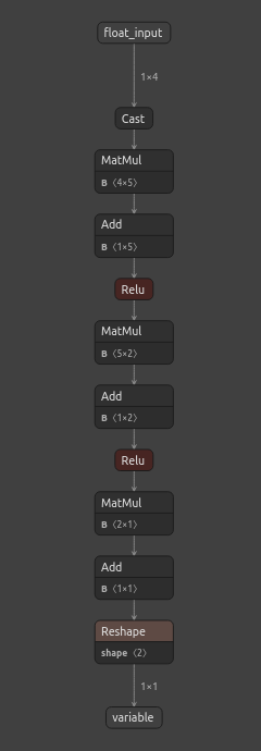
Fig 6: The ONNX representation of our neural network

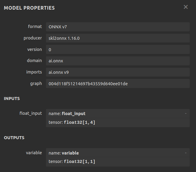
Fig 7: Meta-details of our ONNX model

Netron is an open-source Python library that enables us to visually inspect ONNX models, check their parameters, and review metadata. For those interested in learning more about using ONNX models in MetaTrader 5, there are many well-written articles available. One of my favorite authors on the subject is Omega.

Implementing in MQL5

With our ONNX model's configuration finalized, we can start building our Expert Advisor in MQL5.

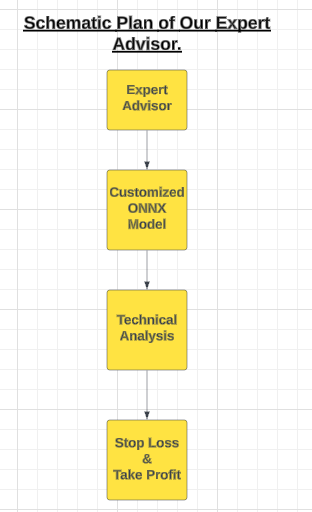
Fig 8: A schematic plan of our Expert Advisor

Our Expert Advisor will use the customized ONNX model to generate entry signals. However, all good traders exercise caution by not executing every entry signal they receive. To instill this discipline in our Expert Advisor, we will program it to wait for confirmation from technical indicators before opening a position.

These technical indicators will help us time our entries effectively. Once positions are open, user-defined stop loss levels will be responsible for closing them. The first step is to specify the ONNX model as a resource for our application.

//+------------------------------------------------------------------+
//|                                   Custom Deep Neural Network.mq5 |
//|                                        Gamuchirai Zororo Ndawana |
//|                                             https://www.mql5.com |
//+------------------------------------------------------------------+
#property copyright "Gamuchirai Zororo Ndawana"
#property link      "https://www.mql5.com/en/gamuchiraindawa"
#property version   "1.00"

//+------------------------------------------------------------------+
//| Load the ONNX model                                              |
//+------------------------------------------------------------------+
#resource "\\Files\\Brent_M1.onnx" as const uchar ModelBuffer[];

Next, we will load the trade library, which is essential for managing our positions.

//+------------------------------------------------------------------+
//| Libraries we need                                                |
//+------------------------------------------------------------------+
#include <Trade/Trade.mqh>
CTrade Trade;

We can now move on to create global variables for our program.

//+------------------------------------------------------------------+
//| Gloabal variables                                                |
//+------------------------------------------------------------------+
long model; //The handler for our ONNX model
vector forecast = vector::Zeros(1); //Our model's forecast

const int states = 3; //The total number of states the system can be in
vector state = vector::Zeros(states); //The state of our system

int mfi_handler,wpr_handler; //Handlers for our technical indicators
vector mfi_reading,wpr_reading; //The values of our indicators will be kept in vectors

double minimum_volume, trading_volume; //Smallest lot size allowed & our calculated lotsize
double ask_price, bid_price; //Market rates

Let us define user inputs that allow us to modify the behavior of the Expert Advisor.

//+------------------------------------------------------------------+
//| Inputs                                                           |
//+------------------------------------------------------------------+
input int mfi_period = 20; //Money Flow Index Period
input int wpr_period = 30; //Williams Percent Range Period

input int lot_multiple = 20; //How big should our lot sizes be?
input double sl_width = 2; //How tight should the stop loss be?

input double max_profit = 10; //Close the position when this profit level is reached.
input double max_loss = 10; //Close the position when this loss level is reached.

Our application requires auxiliary functions to perform specific routines. We begin by defining a function that manages the application's state. This application will have three states: state 0 implies we have no positions, while states 1 and 2 indicate a buy or sell position, respectively.

Depending on the current state, the application will have access to different functions.

//+------------------------------------------------------------------+
//| This function is responsible for updating the system state       |
//+------------------------------------------------------------------+
void update_state(int index)
  {
//--- Reset the system state
   state = vector::Zeros(states);
//--- Now update the current state
   state[index] = 1;
  }

Next, we need a function responsible for validating the user's inputs when starting the application. For example, this function will ensure that all technical indicator periods are greater than 0.

//+------------------------------------------------------------------+
//| This function will ensure that user inputs are valid             |
//+------------------------------------------------------------------+
bool valid_inputs(void)
  {
//--- Let us validate the inputs the user passed
   return((mfi_period > 0)&&(wpr_period > 0) && (max_profit >= 0) && (max_loss >= 0) && (lot_multiple >= 0) && (sl_width >= 0));
  }

Our Expert Advisor will continuously check if the profit levels meet the user's specified inputs. For instance, if the user sets a maximum profit target of $1, the position will be closed automatically once it reaches a $1 profit, even if it hasn't yet reached the take profit level. The same logic applies to stop loss: the position will be closed based on whichever threshold is hit first, whether it's the stop loss level or the maximum loss level. This feature is designed to provide flexibility in defining acceptable risk levels.

//+------------------------------------------------------------------+
//| This function will check our profit levels                       |
//+------------------------------------------------------------------+
void check_profit_level(void)
  {
//--- Let us check if the user set a max profit/loss limit
   if(max_loss > 0 || max_profit > 0)
     {
      //--- If true, let us inspect whether we have passed the limit.
      if((PositionGetDouble(POSITION_PROFIT) > max_profit) || (PositionGetDouble(POSITION_PROFIT) < (max_loss * -1)))
        {
         //--- Close the position
         Trade.PositionClose(Symbol());
        }
     }
  }

Since we have an AI-based system, let's build a function to check if our model forecasts a market move that may be adverse to our open position. Such signals can serve as early indications of changing market sentiment.

//+------------------------------------------------------------------+
//| If we predict a reversal, let's close our positions              |
//+------------------------------------------------------------------+
void find_reversal(void)
  {
//--- We have a position
   if(((state[1] == 1) && (forecast[0] < iClose(Symbol(),PERIOD_CURRENT,0))) || ((state[2] == 1) && (forecast[0] > iClose(Symbol(),PERIOD_CURRENT,0))))
     {
      Trade.PositionClose(Symbol());
     }
  }

Next, we will define a function to check for valid entry signals. An entry signal is considered valid if it meets two conditions: first, it must be supported by price level changes on higher time frames; second, our AI model must forecast a price move aligned with this higher trend. If both conditions are satisfied, we will then check our technical indicators for the final level of confirmation.

//+------------------------------------------------------------------+
//| This function will determine if we have a valid entry            |
//+------------------------------------------------------------------+
void find_entry(void)
  {
//--- First we want to know if the higher timeframes are moving in the same direction we want to go
   double higher_time_frame_trend = iClose(Symbol(),PERIOD_W1,16) - iClose(Symbol(),PERIOD_W1,0);

//--- If price levels appreciated, the difference will be negative
   if(higher_time_frame_trend < 0)
     {
      //--- We may be better off only taking buy opportunities
      //--- Buy opportunities are triggered when the model's prediction is greater than the current price
      if(forecast[0] > iClose(Symbol(),PERIOD_CURRENT,0))
        {
         //--- We will use technical indicators to time our entries
         bullish_sentiment();
        }
     }

//--- If price levels depreciated, the difference will be positive
   if(higher_time_frame_trend > 0)
     {
      //--- We may be better off only taking sell opportunities
      //--- Sell opportunities are triggered when the model's prediction is less than the current price
      if(forecast[0] < iClose(Symbol(),PERIOD_CURRENT,0))
        {
         //--- We will use technical indicators to time our entries
         bearish_sentiment();
        }
     }
  }

Now, we have reached the function responsible for interpreting our technical indicators. There are various ways to interpret these indicators; however, I prefer centering them around 50. By doing so, values greater than 50 confirm bullish sentiment, while values below 50 indicate bearish sentiment. We will use the Money Flow Index (MFI) as our volume indicator and the Williams Percent Range (WPR) as our trend strength indicator.

//+------------------------------------------------------------------+
//| This function will interpret our indicators for buy signals      |
//+------------------------------------------------------------------+
void bullish_sentiment(void)
  {
//--- For bullish entries we want strong volume readings from our MFI
//--- And confirmation from our WPR indicator
   wpr_reading.CopyIndicatorBuffer(wpr_handler,0,0,1);
   mfi_reading.CopyIndicatorBuffer(mfi_handler,0,0,1);
   if((wpr_reading[0] > -50) && (mfi_reading[0] > 50))
     {
      //--- Get the ask price
      ask_price = SymbolInfoDouble(Symbol(),SYMBOL_ASK);
      //--- Make sure we have no open positions
      if(PositionsTotal() == 0)
         Trade.Buy(trading_volume,Symbol(),ask_price,(ask_price - sl_width),(ask_price + sl_width),"Custom Deep Neural Network");
      update_state(1);
     }
  }

//+------------------------------------------------------------------+
//| This function will interpret our indicators for sell signals     |
//+------------------------------------------------------------------+
void bearish_sentiment(void)
  {
//--- For bearish entries we want strong volume readings from our MFI
//--- And confirmation from our WPR indicator
   wpr_reading.CopyIndicatorBuffer(wpr_handler,0,0,1);
   mfi_reading.CopyIndicatorBuffer(mfi_handler,0,0,1);
   if((wpr_reading[0] < -50) && (mfi_reading[0] < 50))
     {
      //--- Get the bid price
      bid_price = SymbolInfoDouble(Symbol(),SYMBOL_BID);
      if(PositionsTotal() == 0)
         Trade.Sell(trading_volume,Symbol(),bid_price,(bid_price + sl_width),(bid_price - sl_width),"Custom Deep Neural Network");
      //--- Update the state
      update_state(2);
     }
  }

Next, we focus on obtaining predictions from our ONNX model. Remember, our model expects inputs of shape [1,4] and returns outputs of shape [1,1]. We define vectors to store the inputs and outputs accordingly, and then use the OnnxRun function to get the model's forecast.

//+------------------------------------------------------------------+
//| This function will fetch forecasts from our model                |
//+------------------------------------------------------------------+
void model_predict(void)
  {
//--- First we get the input data ready
   vector input_data = {iOpen(_Symbol,PERIOD_CURRENT,0),iHigh(_Symbol,PERIOD_CURRENT,0),iLow(_Symbol,PERIOD_CURRENT,0),iClose(_Symbol,PERIOD_CURRENT,0)};
//--- Now we need to perform inferencing
   if(!OnnxRun(model,ONNX_DATA_TYPE_FLOAT,input_data,forecast))
     {
      Comment("Failed to obtain a forecast from the model: ",GetLastError());
      forecast[0] = 0;
      return;
     }
//--- We succeded!
   Comment("Model forecast: ",forecast[0]);
  }

Now we can start building the event handler for our application, which will be invoked upon the initialization of the Expert Advisor. Our procedure will first validate the user inputs, then define the input and output shapes of our ONNX model. Next, we will set up our technical indicators, fetch market data, and finally set the state of our system to 0.

//+------------------------------------------------------------------+
//| Expert initialization function                                   |
//+------------------------------------------------------------------+
int OnInit()
  {
//--- Make sure user inputs are valid
   if(!valid_inputs())
     {
      Comment("Invalid inputs were passed to the application.");
      return(INIT_FAILED);
     }

//--- Create the ONNX model from the buffer
   model = OnnxCreateFromBuffer(ModelBuffer,ONNX_DEFAULT);

//--- Check if we were succesfull
   if(model == INVALID_HANDLE)
     {
      Comment("[ERROR] Failed to create the ONNX model from the buffer: ",GetLastError());
      return(INIT_FAILED);
     }

//--- Set the input shape of the model
   ulong input_shape[] = {1,4};

//--- Check if we were succesfull
   if(!OnnxSetInputShape(model,0,input_shape))
     {
      Comment("[ERROR] Failed to set the ONNX model input shape: ",GetLastError());
      return(INIT_FAILED);
     }

//--- Set the output shape of the model
   ulong output_shape[] = {1,1};

//--- Check if we were succesfull
   if(!OnnxSetOutputShape(model,0,output_shape))
     {
      Comment("[ERROR] Failed to set the ONNX model output shape: ",GetLastError());
      return(INIT_FAILED);
     }

//--- Setup the technical indicators
   wpr_handler = iWPR(Symbol(),PERIOD_CURRENT,wpr_period);
   mfi_handler = iMFI(Symbol(),PERIOD_CURRENT,mfi_period,VOLUME_TICK);

//--- Fetch market data
   minimum_volume = SymbolInfoDouble(Symbol(),SYMBOL_VOLUME_MIN);
   trading_volume = minimum_volume * lot_multiple;

//--- Set the system to state 0, indicating we have no open positions
   update_state(0);

//--- Everything went fine
   return(INIT_SUCCEEDED);
  }

A crucial part of our application is the de-initialization procedure. In this event handler, we will release any resources that are no longer needed when the Expert Advisor is not in use.

//+------------------------------------------------------------------+
//| Expert deinitialization function                                 |
//+------------------------------------------------------------------+
void OnDeinit(const int reason)
  {
//--- Free the onnx resources
   OnnxRelease(model);

//--- Free the indicator resources
   IndicatorRelease(wpr_handler);
   IndicatorRelease(mfi_handler);

//--- Detach the expert advisor
   ExpertRemove();
  }

Finally, we need to define our OnTick event handler. The actions taken will depend on the system's state. If we have no open positions (state 0), our priority will be to obtain a forecast from our model and identify a potential entry. If we have an open position (state 1 for long or state 2 for short), our focus will shift to managing the position. This includes monitoring for potential reversals and checking risk levels, profit targets, and maximum profit levels.

//+------------------------------------------------------------------+
//| Expert tick function                                             |
//+------------------------------------------------------------------+
void OnTick()
  {
//--- Which state is the system in?
   if(state[0] == 1)
     {
      //--- Being in this state means we have no open positions, let's analyse the market to try find one
      model_predict();
      find_entry();
     }

   if((state[1] == 1) || (state[2] == 1))
     {
      //--- Being in this state means we have an position open, if our model forecasts a reversal move we will close
      model_predict();
      find_reversal();
      check_profit_level();
     }
  }
//+------------------------------------------------------------------+

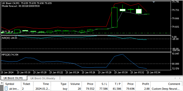
Fig 9: Testing our Expert Advisor

Conclusion

This article provided a gentle introduction to using optimization algorithms for model hyperparameter selection. In future articles, we will adopt a more robust methodology, utilizing two dedicated datasets: one for optimizing the model and the other for cross-validating and comparing its performance against a model using default settings.