Reimagining Classic Strategies: Forecasting Higher Highs And Lower Lows

Introduction

Artificial Intelligence offers possibly infinite opportunities to enhance our trading capabilities. However, it is unlikely that all strategies will be effective. We aim to assist traders in identifying the strategies that best suit their needs by providing the necessary information for informed decision-making.

Given the vast number of potential strategy combinations, no single trader can evaluate them all comprehensively before making important decisions. This pain point is shared by everyone in our trading community. Therefore, throughout this series of articles, we will explore the search space of trading strategies by comparing the accuracy of popular strategies against the simplest models.

In this article, we closely examine the classic price action trading strategy of trading based on “higher highs” or “lower lows.” We trained various models to predict two distinct targets. The first target involved predicting changes in price, the simplest target possible. The second target aimed to determine whether the future close price would be higher than the current high, lower than the current low, or between the two.

To compare models of different complexities, we employed time-series cross-validation without random shuffling. We analyzed the changes in accuracy scores across both targets. Our findings suggest that simpler models, which forecast changes in price levels, may be more effective.

Overview of The Trading Strategy

Typically, when traders following price action strategies analyze a security, they look for signs of strong trends either forming or dying out. A well-known sign of a strong trend forming is when price levels close above previous extreme values and continue to drift away in progressively larger steps. This is colloquially known as "higher highs" or "lower lows." depending on which direction price is moving.

For countless generations, traders have used this simple strategy to identify entry and exit points. Exit points are generally determined when the price fails to break past its extreme values, indicating that the trend is losing strength and may potentially reverse. Over the years, various minor extensions have been added to this strategy, but its fundamental template remains the same.

One of the biggest drawbacks of this strategy is when the price unexpectedly moves back beneath its extreme. These adverse price changes are known as "retracements" and they are difficult to predict. As a result, most traders do not immediately enter a position when the price breaks to a new extreme. Instead, they wait to see how long the price can sustain those levels before committing—essentially allowing the trend to prove itself. However, this approach raises several questions: How long should one wait before concluding that the trend has proven itself? Conversely, how long is too long before the trend reverses? This is the dilemma faced by price action analysts.

Overview of The Methodology

Now that we are familiar with the weaknesses of the trading strategy, we understand the motivation behind employing AI to overcome these past limitations. As mentioned earlier, we trained a diverse group of classifiers to predict whether the price would close beyond its current extreme values or remain within the range. We selected various classifiers, including AdaBoost, decision trees, and neural networks, for this task. No hyperparameter tuning was performed on any of the models before comparison.

We mapped the three potential outcomes to three categorical levels: 1, 2, and 3, respectively:

• 1 represents that the close price in the future will be greater than the high price right now
• 2 represents that the close price in the future will be less than the low price right now
• 3 represents that 1 and 2 were false, the future price will be in-between the current high and low.

It is worth noting that the new target we created is more challenging to interpret. If our model forecasts a transition to state 3, it may remain uncertain whether price levels will appreciate or depreciate, depending on the price at that moment. This makes our model not only less transparent but also seemingly less accurate than the simplest model.

Typically, we award merit to any strategy that can outperform the simplest model. A complex strategy that fails to do so may not justify the additional commitment of constrained resources, such as time.

Exploratory Data Analysis in Python

To kick things off, we first have to export market data from our MetaTrader 5 terminal. We start off by opening the terminal and selecting the Symbol icon. Then select bars from the context menu, search for the symbol you are interested in, and then press export.

Fig 1: Preparing to export market data

Now that our data is ready, let’s start visualizing if there may be any relationships between the variables in question.

We start off by importing the libraries we need.

#import libraries
import pandas as pd
import numpy as np
import seaborn as sns
import matplotlib.pyplot as plt

Then we read in the data we prepared earlier, notice that the MetaTrader 5 terminal gives us csv files that are tab separated. Therefore, we pass the “\t” parameter when reading in the file.

gbpusd = pd.read_csv("/home/volatily/market_data/GBPUSD_Daily_20160103_20240131.csv",sep="\t")

Let us rename the columns in our data-frame.

#Rename the columns
gbpusd.rename(columns={"<DATE>":"Date","<OPEN>":"Open","<HIGH>":"High","<LOW>":"Low","<CLOSE>":"Close","<TICKVOL>":"TickVol","<VOL>":"Vol","<SPREAD>":"Spread"},inplace=True)

Let us define how far ahead into the future we want to forecast.

#Define how far into the future we want to forecast
look_ahead = 20

Now we will define our labels in the same manner we discussed.

#This column will help us with our plots
gbpusd["Future Close"] = gbpusd["Close"].shift(-look_ahead)
#Let's mark the normal target
#If price rises, our target will be 1
#If price falls, our target will be 0
gbpusd["Price Target"] = 0
#Let's mark the new target
#If price makes a higher high, we will label 1
#If price makes a lower low, we will label 2
#If price fails to make either, we will label 3
gbpusd["New Target"] = 0

Labeling the data.

#Labeling the data
#If the future close was less than the current close, price depreciated, label 0
gbpusd.loc[gbpusd["Close"] > gbpusd["Close"].shift(-look_ahead),"Price Target"] = 0
#If the future close was greater than the current close, price depreciated, label 1
gbpusd.loc[gbpusd["Close"] < gbpusd["Close"].shift(-look_ahead),"Price Target"] = 1
#If price makes a higher high our label will be 1
gbpusd.loc[gbpusd["Close"].shift(-look_ahead) > gbpusd["High"],"New Target"] = 1
#If price makes a lower low our label will be 2
gbpusd.loc[gbpusd["Close"].shift(-look_ahead) < gbpusd["Low"],"New Target"] = 2
#Otherwise our label will be 3 
gbpusd.loc[gbpusd["Close"].shift(-look_ahead) < gbpusd["Low"],"New Target"] = 3

We can drop all rows with missing values.

#Drop the last look ahead rows
gbpusd = gbpusd[:-look_ahead]

The trading strategy implies there is a relationship between the close and the high, let us visualize if there is any relationship between the close and the high.

#Plot a scattor plot so we can see if there may be any relationship between the close and the high
sns.scatterplot(data=gbpusd,x="Close",y="High",hue="Price Target")

Fig 2: Visualizing the close plotted against the high

Scatter-plots are helpful because they allow us to visualize relationships between any pair of state variables in the system we are modeling.

By observing the data, we can immediately see what appears to be a strong, almost linear relationship between the close price and the high price. We added color to the plot to distinguish instances where the price appreciated from those where it depreciated. As observed, there is no clear separation between the two instances. The only noticeable separation points appear at extreme values; for example, when the price closes below the 1.1 level, it always seems to bounce back.

We can perform the same scatter-plot, however this time we will place the low price on the y-axis.

#Plot a scattor plot so we can see if there may be any relationship between the close and the low
sns.scatterplot(data=gbpusd,x="Close",y="Low",hue="Price Target")

Fig 3: Visualizing the relationship between the close and the low

As expected, we don’t get much natural separation. This natural separation is desired because it helps our models learn decision boundaries faster. Let us see if our new target helps us to better separate our dataset.

#Plot a scattor plot so we can see if there may be any relationship between the close and the low
sns.scatterplot(data=gbpusd,x="Close",y="Low",hue="New Target")

Fig 4: Our new target doesn't deliver more separation

As we can see, the separation is still poor. The darkest dots, representing state 3, run along almost the entire length of our plot. This is problematic because it visually indicates that there are instances in our data where the same input resulted in different outputs.

To demonstrate what good separation looks like, let's visualize the current price on the x-axis and the future price on the y-axis. We will color the plot points orange for price increases and blue for price decreases.

#Plot a scattor plot so we can see if there may be any relationship between the close and the low
sns.scatterplot(data=gbpusd,x="Close",y="Future Close",hue="Price Target")

Fig 5: A toy example of what good separation looks like

As you can see, there is clear separation between the two classes in this plot. This is to be expected because we are using the target itself in the plot, our goal as machine learning practitioners is to uncover a feature or target that gives us a level of separation that is close to what we see in Fig 4.

If we perform the same plot using our new target, we observe something peculiar.

#Plot a scattor plot so we can see if there may be any relationship between the close and the low
sns.scatterplot(data=gbpusd,x="Close",y="Future Close",hue="New Target")

Fig 6: Visualizing the separation brought about by the new target

Observe that the dark and light points are well separated between the top and bottom halves of the plot, representing instances where the price rose and fell, respectively. Between these two classes, we have points classified as state 3, indicated by the dark spots along the center, showing instances where the price was ranging.

Training The Models

We will now import the models we need and other preprocessing tools.

#Let's get a group of different models
from sklearn.ensemble import RandomForestClassifier
from sklearn.ensemble import BaggingClassifier
from sklearn.ensemble import AdaBoostClassifier
from sklearn.neighbors import KNeighborsClassifier
from sklearn.discriminant_analysis import LinearDiscriminantAnalysis
from sklearn.neural_network import MLPClassifier
from sklearn.svm import LinearSVC
#Import cross validation libraries
from sklearn.model_selection import TimeSeriesSplit
#Import accuracy metrics
from sklearn.metrics import accuracy_score
#Import preprocessors
from sklearn.preprocessing import RobustScaler

We’ll define the parameters for our time series cross validation. Remember that the gap should at least be equal to our forecast horizon.

#Splits
splits = 10
gap = look_ahead

Let us store each of the models we need in a list so that we can programmatically fit all the models we have.

#Store each of the models we need
cols = ["AdaBoostClassifier","Linear DiscriminantAnalysis","Bagging Classifier","Random Forest Classifier","KNeighborsClassifier","Neural Network Small","Neural Network Large"]
models = [AdaBoostClassifier(),LinearDiscriminantAnalysis(),BaggingClassifier(n_jobs=-1),RandomForestClassifier(n_jobs=-1),KNeighborsClassifier(n_jobs=-1),MLPClassifier(hidden_layer_sizes=(5,2),early_stopping=True,max_iter=1000),MLPClassifier(hidden_layer_sizes=(20,10),early_stopping=True,max_iter=1000)]
#Create data frames to store our accuracy with different models on different targets
index = np.arange(0,splits)
price_target = pd.DataFrame(columns=cols,index=index)
new_target = pd.DataFrame(columns=cols,index=index)

We will create our time-series split object for our cross validation test.

#Create the tscv splits
tscv = TimeSeriesSplit(n_splits=splits,gap=gap)

Let us define the predictors and target for our models.

#Define the predictors and target
predictors = ["Open","High","Low","Close"]
target = "New Target"

Performing Cross Validation.

#Now we perform cross validation
for j in (np.arange(len(models))):
    #We need to train each model
    model = models[j]
    for i,(train,test) in enumerate(tscv.split(gbpusd)):
        #Scale the data
        scaler = RobustScaler()
        X_train_scaled = scaler.fit_transform(gbpusd.loc[train[0]:train[-1],predictors])
        scaler = RobustScaler()
        X_test_scaled = scaler.fit_transform(gbpusd.loc[test[0]:test[-1],predictors])
        #Train the model
        model.fit(X_train_scaled,gbpusd.loc[train[0]:train[-1],target])
        #Measure the accuracy
        new_target.iloc[i,j] = accuracy_score(gbpusd.loc[test[0]:test[-1],target],model.predict(X_test_scaled))

Let us observe the performance of each of our models on the simplest target possible.

#Calculate the mean for each column when predicting price 
for i in np.arange(0,len(models)):
    print(f"{cols[i]} achieved accuracy: {price_target.iloc[:,i].mean()}")

AdaBoostClassifier achieved accuracy: 0.5190265486725664
Linear Discriminant Analysis achieved accuracy: 0.5579646017699115
Bagging Classifier achieved accuracy: 0.5075221238938052
Random Forest Classifier achieved accuracy: 0.5349557522123894
KNeighborsClassifier achieved accuracy: 0.536283185840708
Neural Network Small achieved accuracy: 0.45309734513274336
Neural Network Large achieved accuracy: 0.5446902654867257

Linear Discriminant Analysis performed best on this particular dataset, almost attaining 56% accuracy. But let us now see our performance on the new target.

#Calculate the mean for each column when predicting price 
for i in np.arange(0,len(models)):
    print(f"{cols[i]} achieved accuracy: {new_target.iloc[:,i].mean()}")

AdaBoostClassifier achieved accuracy: 0.45929203539823016
Linear DiscriminantAnalysis achieved accuracy: 0.4668141592920355
Bagging Classifier achieved accuracy: 0.4393805309734514
Random Forest Classifier achieved accuracy: 0.45929203539823016
KNeighborsClassifier achieved accuracy: 0.465929203539823
Neural Network Small achieved accuracy: 0.3920353982300885
Neural Network Large achieved accuracy: 0.4606194690265487

LDA was still top of our list in both instances. All the models demonstrated weaker skill on the new target, but the small neural network suffered the biggest drop in performance.

Model	Change In Performance
AdaBoostClassifier	-14.32748538011695%
Linear Discriminant Analysis	-19.526066350710863%
Bagging Classifier	-22.09660842754366%
Random Forest Classifier	-16.730769230769248%
KNeighborsClassifier	-15.099715099715114%
Neural Network Small	-41.04193138500632%
Neural Network Large	-21.1502782931354%

Let’s analyze the confusion matrix of our best performing model.

#Let's continue analysing the performance of our best model Linear Discriminant Analysis
from mlxtend.evaluate import confusion_matrix
from mlxtend.plotting import plot_confusion_matrix
model = LinearDiscriminantAnalysis()
model.fit(gbpusd.loc[0:1000,predictors],gbpusd.loc[0:1000,"New Target"])
cm = confusion_matrix(y_target=gbpusd.loc[1000:,"New Target"],y_predicted=model.predict(gbpusd.loc[1000:,predictors]),binary=True)
fig , ax = plot_confusion_matrix(cm)

Fig 7: The confusion matrix for our LDA model

The confusion matrix helps us identify which classes are challenging for our model. As shown in the plot above, our model performed worst when forecasting class 3. However, this class has a small set of observations. To address this, we may need to use data that better represents the entire population. We can achieve this by fetching more historical data or analyzing lower time-frames.

Feature Selection

Sometimes, we can improve performance by dropping unnecessary features from our models. Let's focus on our best-performing model, LDA, and identify its most important features to see if we can enhance performance further.

#Now let us perform feature selection
from mlxtend.feature_selection import SequentialFeatureSelector

There are many feature selection algorithms available, and in this article, we used the forward feature selection algorithm. While there are various versions of this algorithm, the general process starts with a null model that serves as a benchmark. The algorithm then evaluates each of the p available features one by one, selecting the one that produces the greatest performance improvement as the first feature. This process is repeated for the remaining p-1 predictors. Thanks to recent advances in parallel computation, such algorithms have become more feasible.

By reducing our predictors from p to k, where k<p, and choosing the k features wisely, we may be able to either outperform our original model or achieve a model that is equally reliable but faster to train. Furthermore, reducing the number predictors used in the model can reduce the variance of our model's coefficients.

However, there are 2 strong limitations of this algorithm worth discussing. First, the new model may be slightly more biased due to the limited information we are using to train it. Furthermore, the choice of the first feature influences subsequent selections. If the initial feature chosen has little relationship with the target, subsequent features may appear uninformative due to this initial poor choice.

In our analysis, we allowed the feature selector to choose as many variables as it deemed important, but it selected only one: the open price.

#Forward feature selection 
forward_feature_selection = SequentialFeatureSelector(LinearDiscriminantAnalysis(),
                                                     k_features =(1,4),
                                                     forward=True,
                                                     verbose=2,
                                                     scoring="accuracy",
                                                     cv=5,
                                                     n_jobs=-1).fit(gbpusd.loc[:,predictors],gbpusd.loc[:,"New Target"])

Now we want to see the best feature.

#Best feature
forward_feature_selection.k_feature_names_

(Open,)

Let’s observe our new accuracy levels.

#Update the predictors and target
predictors = ["Open"]
target = "New Target"
best_features_for_new_target = pd.DataFrame(columns=["Linear Discriminant Analysis"],index=index)

Perform cross validation using the best feature we identified.

#Now we perform cross validation
for i,(train,test) in enumerate(tscv.split(gbpusd)):
    #First initialize the model
    model = LogisticRegression()
    #Train the model
    model.fit(gbpusd.loc[train[0]:train[-1],predictors],gbpusd.loc[train[0]:train[-1],target])
    #Measure the accuracy
    best_features_for_new_target.iloc[i,0] = accuracy_score(gbpusd.loc[test[0]:test[-1],target],model.predict(gbpusd.loc[test[0]:test[-1],predictors]))

Let us observe our new accuracy levels.

#New accuracy only using the open price
best_features_for_new_target.iloc[:,0].mean()

0.46548672566371685

And finally, let us observe the change in performance between the model that used all the predictors and the model that only used one.

-0.0013274336283186638

As we can see the change in performance is about -0.2%. Meaning we lost very little information by letting go of the other 3 predictors.

Implementing the strategy in MQL5

We start off by importing the libraries we need.

//+------------------------------------------------------------------+
//|                                   Forecasting Highs And Lows.mq5 |
//|                                        Gamuchirai Zororo Ndawana |
//|                                             https://www.mql5.com |
//+------------------------------------------------------------------+
#property copyright "Gamuchirai Zororo Ndawana"
#property link      "https://www.mql5.com"
#property version   "1.00"

//+------------------------------------------------------------------+
//|Libraries we need                                                 |
//+------------------------------------------------------------------+
#include <Trade/Trade.mqh> //Trade class
CTrade Trade;             //Initialize the class

Then we define input variables, so our end user can customize his experience.

//+------------------------------------------------------------------+
//| Input variables                                                  |
//+------------------------------------------------------------------+
input int fetch = 10; //How much data should we fetch?
input int look_ahead = 2; //Forecst horizon.
input int rsi_period = 20; //Forecst horizon.
int input  lot_multiple = 1; //How many times bigger than minimum lot?
input double stop_loss_values = 1; //How large should our stop loss be?

We need some global variables that will be used throughout our application.

//+------------------------------------------------------------------+
//| Global variables                                                 |
//+------------------------------------------------------------------+
vector state = vector::Zeros(3);//This vector will store the state of the system using binary mapping
double minimum_volume;//The smallest contract size allowed
vector input_data;//Input data
vector output_data;//Output data
vector rsi_data;//RSI output data
double variance;//This is the variance of our input data
int classes = 3;//The total number of output classes we have
vector mean_values = vector::Zeros(classes);//This vector will store the mean value for each class
vector probability_values = vector::Zeros(classes);//This vector will store the prior probability the target will belong each class
vector total_class_count = vector::Zeros(classes);//This vector will count the number of times each class was the target
int rsi_handler;//This will store our RSI handler
int forecast = 0;//Our model's forecast
double discriminant_values[3];//The discriminant function

Then we shall define the initialization procedure for our Expert Advisor. Our procedure first ensures that the user passed valid inputs, and then proceeds to set up our technical indicator and initializes the state of our trading system.

//+------------------------------------------------------------------+
//| Expert initialization function                                   |
//+------------------------------------------------------------------+
int OnInit()
  {
//--- Validate inputs
   if(!valid_inputs())
     {
      //User passed invalid inputs
      Print("Invalid inputs were received!");
      return(INIT_FAILED);
     }
//--- Load input data
   rsi_handler = iRSI(_Symbol,PERIOD_CURRENT,rsi_period,PRICE_CLOSE);
//--- Market data
   minimum_volume = SymbolInfoDouble(_Symbol,SYMBOL_VOLUME_MIN);
//--- Update system state
   update_system_state(0);
//--- End of initialization
   return(INIT_SUCCEEDED);
  }

We also need to define a de-initialization procedure for our application.

//+------------------------------------------------------------------+
//| Expert deinitialization function                                 |
//+------------------------------------------------------------------+
void OnDeinit(const int reason)
  {
//--- Remove indicators
   IndicatorRelease(rsi_handler);
//--- Detach the Expert Advisor
   ExpertRemove();
//--- End of deinitialization
  }

We will build out a function to help us analyzes whether we have any entry signals, our entry signals are considered valid if the model’s forecast aligns with the trend on higher time frames, such as the weekly. If the two do align, we will time our entries using the RSI indicator.

//+------------------------------------------------------------------+
//| This function will analyse our entry signals                     |
//+------------------------------------------------------------------+
void analyse_entry(void)
  {
   Print("Higher Time Frame Trend");
   Print(iClose(_Symbol,PERIOD_W1,12) - iClose(_Symbol,PERIOD_CURRENT,0));
   if(iClose(_Symbol,PERIOD_W1,12) < iClose(_Symbol,PERIOD_CURRENT,0))
     {

      if(forecast == 1)
        {
         bullish_sentiment();
        }
     }
   if(iClose(_Symbol,PERIOD_W1,12) > iClose(_Symbol,PERIOD_CURRENT,0))
     {

      if(forecast == 2)
        {
         bearish_sentiment();
        }
     }
  }

We need two dedicated functions for interpreting our RSI indicator, one function will analyze the indicator for sell opportunities and the other for buy opportunities.

//+------------------------------------------------------------------+
//| This function will analyze our RSI for sell signals              |
//+------------------------------------------------------------------+
void bearish_sentiment(void)
  {
   rsi_data.CopyIndicatorBuffer(rsi_handler,0,0,1);
   if(rsi_data[0] < 50)
     {
      Trade.Sell(minimum_volume * lot_multiple,_Symbol,SymbolInfoDouble(_Symbol,SYMBOL_BID),(SymbolInfoDouble(_Symbol,SYMBOL_BID) + stop_loss_values),(SymbolInfoDouble(_Symbol,SYMBOL_BID) - stop_loss_values));
      update_system_state(2);
     }
  }
//+------------------------------------------------------------------+
//| This function will analyze our RSI for buy signals               |
//+------------------------------------------------------------------+
void bullish_sentiment(void)
  {
   rsi_data.CopyIndicatorBuffer(rsi_handler,0,0,1);
   if(rsi_data[0] > 50)
     {
      Trade.Buy(minimum_volume * lot_multiple,_Symbol,SymbolInfoDouble(_Symbol,SYMBOL_ASK),(SymbolInfoDouble(_Symbol,SYMBOL_ASK) - stop_loss_values),(SymbolInfoDouble(_Symbol,SYMBOL_ASK) +stop_loss_values));
      update_system_state(2);
     }
  }

We shall now define a function that will validate the inputs our user passed upon initialization.

//+------------------------------------------------------------------+
//|This function will check the inputs the user passed               |
//+------------------------------------------------------------------+
bool valid_inputs(void)
  {
//--- For the inputs to be valid:
//--- The forecast horizon must be less than the data fetched
   return((fetch > look_ahead));
  }

Let us now design a function that will initialize our LDA model.

//+------------------------------------------------------------------+
//| This function will initialize our model                          |
//+------------------------------------------------------------------+
void initialize_model(void)
  {
//--- First fetch the input data
   fetch_input_data(look_ahead,fetch);
   fetch_output_data(0,fetch);
//--- Update the system state
   update_system_state(1);
//--- Fit the model
   fit_model();
  }

To initialize the model, we need to first fetch input data for the model, that is the responsibility of this function. Note that the function simply fetches the open price because our analysis suggested that it was the most important feature we had.

//+------------------------------------------------------------------+
//| This function will fetch our input data                          |
//+------------------------------------------------------------------+
void fetch_input_data(int start,int size)
  {
//--- Fetching input data
   Print("Fetching input data");
   input_data = vector::Zeros(fetch);
   input_data.CopyRates(_Symbol,PERIOD_CURRENT,COPY_RATES_OPEN,start,size);
   input_data.Resize(size);
   Print("Input data fetched");
  }

Then we need to fetch our output data and label it, also note that we keep track of how many times each class appeared as the target, this information will be used later on when we are fitting the LDA model.

//+------------------------------------------------------------------+
//| This function will fetch our output data                         |
//+------------------------------------------------------------------+
void fetch_output_data(int start,int size)
  {
//--- Fetching output data
   vector historic_high = vector::Zeros(size);
   vector historic_low = vector::Zeros(size);
   vector historic_close = vector::Zeros(size);
   historic_close.CopyRates(_Symbol,PERIOD_CURRENT,COPY_RATES_CLOSE,start,size+look_ahead);
   historic_low.CopyRates(_Symbol,PERIOD_CURRENT,COPY_RATES_HIGH,start,size+look_ahead);
   historic_high.CopyRates(_Symbol,PERIOD_CURRENT,COPY_RATES_LOW,start,size+look_ahead);
   output_data = vector::Zeros(size);
   output_data.Resize(size);
//--- Reset class counts
   total_class_count[0] = 0;
   total_class_count[1] = 0;
   total_class_count[2] = 0;
//--- Label the data
   for(int i = 0; i < size; i++)
     {
      //--- Price broke into a higher high
      if(historic_close[i + look_ahead] > historic_high[i])
        {
         output_data[i] = 1;
         total_class_count[0] += 1;
        }
      //--- Price broke into a lower low
      else
         if(historic_close[i + look_ahead] < historic_low[i])
           {
            output_data[i] = 2;
            total_class_count[1] += 1;
           }
         //--- Price was stuck in a range
         else
            if((historic_close[i + look_ahead] > historic_low[i]) && (historic_close[i + look_ahead] < historic_high[i]))
              {
               output_data[i] = 3;
               total_class_count[2] += 1;
              }
     }
//--- We fetched output data succesfully
   Print("Output data fetched");
   Print("Total class counts");
   Print(total_class_count);
  }

Now we define the procedure for fitting the LDA model. The first step involves us calculating the average value of the Open price in each of the 3 classes. The second steps require us to calculate the prior probability distribution of each class being the target class, we can simply estimate this value by using the class counts we performed in the previous step. Lastly, we need to calculate the variance of the Open price for each of the 3 classes.

//+------------------------------------------------------------------+
//| This function will fit the LDA algorithm                         |
//+------------------------------------------------------------------+
//--- Fit the model
void fit_model(void)
  {
//--- To fit the LDA model, we first need to know the mean value of X for each of our 3 classes
   double sum_class_one = 0;
   double sum_class_two = 0;
   double sum_class_three = 0;

//--- In this case we only have 1 input
   for(int i = 0; i < fetch;i++)
     {
      //--- Class 1
      if(output_data[i] == 1)
        {
         sum_class_one += input_data[i];
        }
      //--- Class 2
      else
         if(output_data[i] == 2)
           {
            sum_class_two += input_data[i];
           }
         //--- Class 3
         else
            if(output_data[i] == 3)
              {
               sum_class_three += input_data[i];
              }
     }
//--- Calculate the mean value for each class
   mean_values[0] = sum_class_one / total_class_count[0];
   mean_values[1] = sum_class_two / total_class_count[1];
   mean_values[2] = sum_class_three / total_class_count[2];
   Print("Mean values");
   Print(mean_values);
//--- Now we need to calculate class probabilities
   for(int i=0;i<classes;i++)
     {
      probability_values[i] = total_class_count[i] / fetch;
     }
   Print("Class probability values");
   Print(probability_values);
//--- Calculating the variance
   Print("Calculating the variance");
//--- Next we need to calculate the variance of the inputs within each class of y.
//--- This process can be simplified into 2 steps
//--- First we calculate the difference of each instance of x from the group mean.
   double squared_difference[3];
   for(int i =0; i < fetch;i++)
     {
      //--- If the output value was 1, find the input value that created the output
      //--- Calculate how far that value is from it's group mean and square the difference
      if(output_data[i] == 1)
        {
         squared_difference[0] = MathPow((input_data[i]-mean_values[0]),2);
        }

      else
         if(output_data[i] == 2)
           {
            squared_difference[1] = MathPow((input_data[i]-mean_values[1]),2);
           }

         else
            if(output_data[i] == 3)
              {
               squared_difference[2] = MathPow((input_data[i]-mean_values[2]),2);
              }
     }
//--- Show the squared difference values
   Print("Squared difference value for each output value of y");
   ArrayPrint(squared_difference);

//--- Next we calculate the variance as the average squared difference from the mean
   variance = (1.0/(fetch - 3.0)) * (squared_difference[0] + squared_difference[1] + squared_difference[2]);
   Print("Variance: ",variance);
  }

Now we need a function to fetch forecasts from our model, our model will forecast a discriminant value for each of the 3 possible classes. The class with the largest discriminant value is the predicted class.

//+-------------------------------------------------------------------+
//| This model will fetch our model's prediction                      |
//+-------------------------------------------------------------------+
void model_forecast(void)
  {
//--- Obtain a forecast from our model
//--- First we need to fetch the most recent input data
   fetch_input_data(0,1);
//--- We need to calculate the discriminant function for each class
//--- The predicted class is the one with the largest discriminant function
   Print("Calculating discriminant values.");
   for(int i = 0; i < classes; i++)
     {
      discriminant_values[i] = (input_data[0] * (mean_values[i]/variance) - (MathPow(mean_values[i],2)/(2*variance)) + (MathLog(probability_values[i])));
     }
//--- Show the LDA prediction
   forecast = (ArrayMaximum(discriminant_values) +1);
   Print("LDA Forecast: ",forecast);
   ArrayPrint(discriminant_values);
  }

We need a function to update the state of our system so that our OnTick function will always know what to do next.

//+-------------------------------------------------------------------+
//| This function will be used to update the state of the system      |
//+-------------------------------------------------------------------+
void update_system_state(int index)
  {
//--- Each column vector is set to 0 except column 0, the first column.
//--- If the first column is set to 1, then our model has not been trained
//--- If the second column is set to 1, then our model has been trained but we have no positions
//--- If the third column is set to 1, then we have a position we need to manage
//--- Update the system state
   state = vector::Zeros(3);
   state[index] = 1;
   Print("Updating system state");
   Print(state);
  }

Let us now define the OnTick function, that will ensure all our functions are called at the appropriate time.

//+------------------------------------------------------------------+
//| Expert tick function                                             |
//+------------------------------------------------------------------+
void OnTick()
  {
//--- The model has not been trained
   if(state.ArgMax() == 0)
     {
      Print("Training the model.");
      initialize_model();
     }
//--- The model has been trained, but we have no positions
   else
      if(state.ArgMax() == 1)
        {
         Print("Finding An Entry.");
         model_forecast();
         analyse_entry();
        }
  }
//+------------------------------------------------------------------+

Fig8: Our expert advisor

Fig 9: Our LDA Expert Advisor

 

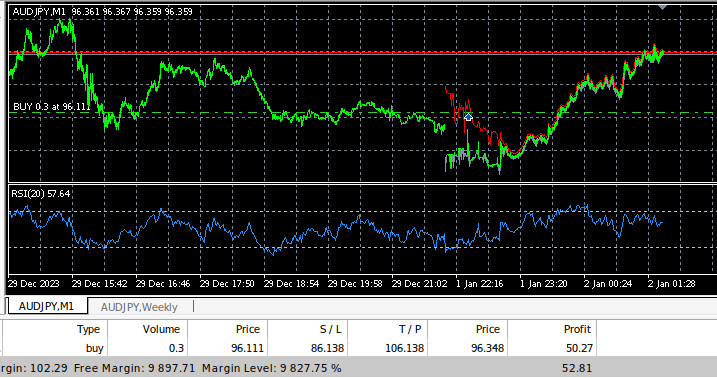
Fig 10: Our Expert Advisor trading historical data

Conclusion

In this article, we have demonstrated why it appears that traders may be better off forecasting changes in price than they are forecasting higher highs and lower lows, hopefully after reading this article you will have more confidence in deciding if this trading strategy is suitable for you, given your personal levels of risk tolerance and your financial goals.

The Linear Discriminant Analysis (LDA) algorithm models the distribution of input variables within each class, using Bayes' Theorem to estimate probabilities and assuming normal distribution with class-specific means and common variance. This helps LDA effectively distinguish class characteristics by calculating discriminant values that maximize class separation and minimize within-class variance. However, LDA's assumptions can limit transparency and interpretability, and it may underperform simpler models without extensive parameter tuning. Our tests using default settings on daily data revealed potential performance issues, suggesting that better results might be achieved with more data and computational resources.

Repeating the analysis with larger datasets could provide more insights, though this approach is feasible only with sufficient computational power. We used 10-fold time-series cross-validation, which means each model was trained 10 times. As the dataset size increases, one might expect model training times to grow exponentially.