Data Science and ML (Part 31): Using CatBoost AI Models for Trading

MetaTrader 5 — Trading | 15 October 2024, 15:49

1 887

"CatBoost is a gradient boosting library that distinguishes itself by handling categorical features in an efficient and scalable way, providing a significant performance boost for many real-world problems."

— Anthony Goldbloom.

What is CatBoost?

CatBoost is an open-source software library with gradient-boosting algorithms on decision trees, it was designed specifically to address the challenges of handling categorical features and data in machine learning.

It was developed by Yandex and was made open-source in the year of 2017, read more.

Despite being introduced recently compared to machine learning techniques such as Linear regression or SVM's, CatBoost gained massive popularity among AI communities and rose to the top of the most used machine learning models on platforms like Kaggle.

What made CatBoost gain this much attention is its ability to automatically handle categorical features in the dataset, which can be challenging to many machine learning algorithms.

Catboost models usually provide a better performance compared to other models with minimal effort, even with the default parameters and settings, these models can perform well accuracy-wise.
Unlike neural networks which require domain knowledge to code and make themwork, CatBoost's implementation is straightforward.

This article assumes that you have a basic understanding of machine learning, Decision Trees, XGBoost, LightGBM, and ONNX.

How Does CatBoost Operate?

CatBoost is based on a gradient boosting algorithm just like Light Gradient Machine (LightGBM) and Extreme Gradient Boosting (XGBoost). It works by building several decision tree models sequentially where each model builds on the previous one as it tries to correct the error of previous models.

The final prediction is a weighted sum of the predictions made by all the models involved in the process.

The objective of these Gradient Boosted Decision Trees (GBDTs) is to minimize to minimize the loss function, this is done by adding a new model that corrects the previous model's mistakes.

Handling categorical features

As I explained earlier, CatBoost has can handle categorical features without the need for explicit encoding like One-hot encoding or label encoding which is required for other machine learning models, This is because; CatBoost introduces target-based encoding for categorical features.

This encoding is performed by computing a conditional distribution of the target for each categorical feature value.

Another key innovation in CatBoost is using ordered boosting when computing the statistics for categorical features. This ordered boosting ensures the encoding for any instance is based on the information from previously observed data points.

This helps to avoid data leakage and to avoid overfitting.

It uses Symmetric Decision Tree Structures

Unlike LightGBM and XGBoost which uses asymmetric trees, CatBoost uses symmetric decision trees for the decision-making process. In a symmetric tree, both left and right branches at each split are constructed symmetrically based on the same splitting rule, this approach has several advantages such as;

It leads to faster training since both splits are symmetrical.
Efficient memory usage due to the easier tree structure.
Symmetrical trees are more robust to small perturbations in the data.

CatBoost vs XGBoost and LightGBM, A Detailed Comparison

Let's understand how CatBoost differs from other Gradient-boosted decision trees. Let's understand the differences between these three, this way we know when to use one among these three and when not to.

Aspect	CatBoost	LightGBM	XGBoost
Categorical features handling	Equipped with automatic encoding and ordered boosting for handling categorical variables.	Requires manual encoding processing such as one-hot encoding, label encoding, etc.	Requires manual encoding processing such as one-hot encoding, label encoding, etc.
Decision Tree Structure	It has symmetric decision trees, which are balanced and grow evenly. They ensure faster predictions and a lower risk of overfitting.	It has a Leaf-wise growth strategy (asymmetric) which focuses on the leaves with the highest loss. This results in deep and imbalanced trees which can carry a higher accuracy but, a greater risk of overfitting.	It has a Level-wise growth strategy (asymmetric) which grows the tree based on the best split for each node. This leads to flexible but slower predictions and a potential risk of overfitting.
Model accuracy	They provide good accuracy when working with datasets containing many categorical features due to ordered boosting and reduced risk of overfitting on smaller data.	They provide good accuracy, particularly on large and high-dimensional datasets since the leaf-wise growth strategy focuses on improving performance in areas of high error.	They provide good accuracy on most datasets but, tend to be outperformed by CatBoost on categorical datasets and LightGBM on very large datasets due to its less aggressive tree-growing strategy.
Training speed & accuracy	Usually slower to train than LightGBM but more efficient on small to medium datasets, especially when categorical features are involved.	Usually the fastest of these three, especially on large datasets due to its leaf-wise tree growth which is more efficient in high-dimensional data.	Often the slowest of these three by a tiny margin. It is very efficient for large datasets.

Deploying a CatBoost Model

Before we can write code for CatBoost, let us create a problem scenario. We want to predict the trading signals (Buy/ Sell) using the data; Open, High, Low, Close and a couple of categorical features such as Day (which is the current date), day of week (from Monday to Sunday), Day of year (from 1 to 365), and the Month (from January to December).

The OHLC (Open, High, Low, Close) values are continuous features while the rest are categorical features. A script to collect this data can be located in attachments.

We start by importing the CatBoost model after installing it.

Installing

Command Line

pip install catboost

Importing.

Python code

import numpy as np
import pandas as pd
import catboost
from catboost import CatBoostClassifier
from sklearn.pipeline import Pipeline 
from sklearn.model_selection import train_test_split
from sklearn.metrics import classification_report
import seaborn as sns
import matplotlib.pyplot as plt

sns.set_style("darkgrid")

We can visualize the data to see what is it all about.

df = pd.read_csv("/kaggle/input/ohlc-eurusd/EURUSD.OHLC.PERIOD_D1.csv")

df.head()

Outcome

	Open	High	Low	Close	Day	DayofWeek	DayofYear	Month
0	1.09381	1.09548	1.09003	1.09373	21.0	3.0	264.0	9.0
1	1.09678	1.09810	1.09361	1.09399	22.0	4.0	265.0	9.0
2	1.09701	1.09973	1.09606	1.09805	23.0	5.0	266.0	9.0
3	1.09639	1.09869	1.09542	1.09742	26.0	1.0	269.0	9.0
4	1.10302	1.10396	1.09513	1.09757	27.0	2.0	270.0	9.0

While collecting data inside an MQL5 script, I obtained the values DayofWeek (Monday to Sunday) and Month (January - December) as integers instead of strings since I was storing them in a matrix which wouldn't allow me to add strings, despite them being categorical variables by nature as it stands now they are not, we are going to convert them into categories again and see how CatBoost can handle them.

Let us prepare the target variable.

Python code

new_df = df.copy()  # Create a copy of the original DataFrame

# we Shift the 'Close' and 'open' columns by one row to ge the future close and open price values, then we add these new columns to the dataset

new_df["target_close"] = df["Close"].shift(-1)  
new_df["target_open"] = df["Open"].shift(-1)  

new_df = new_df.dropna()  # Drop the rows with NaN values resulting from the shift operation

open_values = new_df["target_open"]
close_values = new_df["target_close"]  

target = []
for i in range(len(open_values)):
    if close_values[i] > open_values[i]: 
        target.append(1) # buy signal 
    else:
        target.append(0) # sell signal

new_df["signal"] = target # we create the signal column and add the target variable we just prepared


print(new_df.shape)
new_df.head()

Outcome

	Open	High	Low	Close	Day	DayofWeek	DayofYear	Month	target_close	target_open	signal
0	1.09381	1.09548	1.09003	1.09373	21.0	3.0	264.0	9.0	1.09399	1.09678	0
1	1.09678	1.09810	1.09361	1.09399	22.0	4.0	265.0	9.0	1.09805	1.09701	1
2	1.09701	1.09973	1.09606	1.09805	23.0	5.0	266.0	9.0	1.09742	1.09639	1
3	1.09639	1.09869	1.09542	1.09742	26.0	1.0	269.0	9.0	1.09757	1.10302	0
4	1.10302	1.10396	1.09513	1.09757	27.0	2.0	270.0	9.0	1.10297	1.10431	0

Now that we have the signals we can predict, let us split the data into training and testing samples.

X = new_df.drop(columns = ["target_close", "target_open", "signal"]) # we drop future values
y = new_df["signal"] # trading signals are the target variables we wanna predict 

X_train, X_test, y_train, y_test = train_test_split(X, y, train_size=0.7, random_state=42)

We define a list of categorical features present in our dataset.

categorical_features = ["Day","DayofWeek", "DayofYear", "Month"]

We can then use this list to convert these categorical features into strings format, since categorical variables are usually in strings format.

X_train[categorical_features] = X_train[categorical_features].astype(str)
X_test[categorical_features] = X_test[categorical_features].astype(str)

X_train.info() # we print the data types now

Outcome

<class 'pandas.core.frame.DataFrame'>
Index: 6999 entries, 9068 to 7270
Data columns (total 8 columns):
 #   Column     Non-Null Count  Dtype  
---  ------     --------------  -----  
 0   Open       6999 non-null   float64
 1   High       6999 non-null   float64
 2   Low        6999 non-null   float64
 3   Close      6999 non-null   float64
 4   Day        6999 non-null   object 
 5   DayofWeek  6999 non-null   object 
 6   DayofYear  6999 non-null   object 
 7   Month      6999 non-null   object 
dtypes: float64(4), object(4)
memory usage: 492.1+ KB

We now have categorical variables with object data types, which are strings data types. If you try this data to a machine learning model other than CatBoost you will get errors since objects data types are not allowed in a typical machine learning training data.

Training a CatBoost Model

Before calling the fit method, which is responsible for training the CatBoost model, let's understand a few of the many parameters that make this model tick.

Parameter	Description
Iterations	This is the number of decision trees iterations to build. More iterations lead to better performance but also carry a risk of overfitting.
learning_rate	This factor controls the distribution of each tree to the final prediction. A smaller learning rate requires more iterations for trees to converge but often results in better models.
depth	This is the maximum depth of the trees. Deeper trees can capture more complex patterns in the data but, may often lead to overfitting.
cat_features	This is a list of categorical indices. Despite the CatBoost model being capable of detecting the categorical features, it is a good practice to explicitly instruct the model on which features are categorical ones. This helps the model understand the categorical features from a human perspective as the methods for automatically detecting the categorical variables can sometimes fail.
l2_leaf_reg	This is the L2 regularization coefficient. It helps to prevent overfitting by penalizing larger leaf weights.
border_count	This is the number of splits for each categorical feature. The higher this number the better the performance and increases computational time.
eval_metric	This is the evaluation metric that will be used during training. It helps in monitoring the model performance effectively.
early_stopping_rounds	When validation data is provided to the model, the training progress will stop if no improvement in the model's accuracy is observed for this number of rounds. This parameter helps reduce overfitting and can save a lot of training time.

We can define a dictionary for the above parameters.

params = dict(
    iterations=100, 
    learning_rate=0.01,
    depth=10,
    l2_leaf_reg=5,  
    bagging_temperature=1,
    border_count=64,  # Number of splits for categorical features
    eval_metric='Logloss',
    random_seed=42,  # Seed for reproducibility
    verbose=1,  # Verbosity level
    # early_stopping_rounds=10  # Early stopping for validation
)

Finally, we can define the Catboost model inside the Sklearn pipeline, then call the fit method for training giving this method evaluation data and a list of categorical features.

pipe = Pipeline([
    ("catboost", CatBoostClassifier(**params))
])

# Fit the pipeline to the training data
pipe.fit(X_train, y_train, catboost__eval_set=(X_test, y_test), catboost__cat_features=categorical_features)

Outputs

90:     learn: 0.6880592        test: 0.6936112 best: 0.6931239 (3)     total: 523ms    remaining: 51.7ms
91:     learn: 0.6880397        test: 0.6936100 best: 0.6931239 (3)     total: 529ms    remaining: 46ms
92:     learn: 0.6880350        test: 0.6936051 best: 0.6931239 (3)     total: 532ms    remaining: 40ms
93:     learn: 0.6880280        test: 0.6936103 best: 0.6931239 (3)     total: 535ms    remaining: 34.1ms
94:     learn: 0.6879448        test: 0.6936110 best: 0.6931239 (3)     total: 541ms    remaining: 28.5ms
95:     learn: 0.6878328        test: 0.6936387 best: 0.6931239 (3)     total: 547ms    remaining: 22.8ms
96:     learn: 0.6877888        test: 0.6936473 best: 0.6931239 (3)     total: 553ms    remaining: 17.1ms
97:     learn: 0.6877408        test: 0.6936508 best: 0.6931239 (3)     total: 559ms    remaining: 11.4ms
98:     learn: 0.6876611        test: 0.6936708 best: 0.6931239 (3)     total: 565ms    remaining: 5.71ms
99:     learn: 0.6876230        test: 0.6936898 best: 0.6931239 (3)     total: 571ms    remaining: 0us

bestTest = 0.6931239281
bestIteration = 3

Shrink model to first 4 iterations.

Evaluating the Model

We can use Sklearn metrics to evaluate this model's performance.

# Make predicitons on training and testing sets
y_train_pred = pipe.predict(X_train)
y_test_pred = pipe.predict(X_test)

# Training set evaluation
print("Training Set Classification Report:")
print(classification_report(y_train, y_train_pred))

# Testing set evaluation
print("\nTesting Set Classification Report:")
print(classification_report(y_test, y_test_pred))

Outputs

Training Set Classification Report:
              precision    recall  f1-score   support

           0       0.55      0.44      0.49      3483
           1       0.54      0.64      0.58      3516

    accuracy                           0.54      6999
   macro avg       0.54      0.54      0.54      6999
weighted avg       0.54      0.54      0.54      6999


Testing Set Classification Report:
              precision    recall  f1-score   support

           0       0.53      0.41      0.46      1547
           1       0.49      0.61      0.54      1453

    accuracy                           0.51      3000
   macro avg       0.51      0.51      0.50      3000
weighted avg       0.51      0.51      0.50      3000

The outcome is an average performing model. I realized after removing the categorical features list the model accuracy rose to 60% on the training set, but it remained the same on the testing set.

pipe.fit(X_train, y_train, catboost__eval_set=(X_test, y_test))

Outcome

91:     learn: 0.6844878        test: 0.6933503 best: 0.6930500 (30)    total: 395ms    remaining: 34.3ms
92:     learn: 0.6844035        test: 0.6933539 best: 0.6930500 (30)    total: 399ms    remaining: 30ms
93:     learn: 0.6843241        test: 0.6933791 best: 0.6930500 (30)    total: 404ms    remaining: 25.8ms
94:     learn: 0.6842277        test: 0.6933732 best: 0.6930500 (30)    total: 408ms    remaining: 21.5ms
95:     learn: 0.6841427        test: 0.6933758 best: 0.6930500 (30)    total: 412ms    remaining: 17.2ms
96:     learn: 0.6840422        test: 0.6933796 best: 0.6930500 (30)    total: 416ms    remaining: 12.9ms
97:     learn: 0.6839896        test: 0.6933825 best: 0.6930500 (30)    total: 420ms    remaining: 8.58ms
98:     learn: 0.6839040        test: 0.6934062 best: 0.6930500 (30)    total: 425ms    remaining: 4.29ms
99:     learn: 0.6838397        test: 0.6934259 best: 0.6930500 (30)    total: 429ms    remaining: 0us

bestTest = 0.6930499562
bestIteration = 30

Shrink model to first 31 iterations.

Training Set Classification Report:
              precision    recall  f1-score   support

           0       0.61      0.53      0.57      3483
           1       0.59      0.67      0.63      3516

    accuracy                           0.60      6999
   macro avg       0.60      0.60      0.60      6999
weighted avg       0.60      0.60      0.60      6999

To understand this model further in detail, let us create the feature importance plot.

# Extract the trained CatBoostClassifier from the pipeline
catboost_model = pipe.named_steps['catboost']

# Get feature importances
feature_importances = catboost_model.get_feature_importance()

feature_im_df = pd.DataFrame({
    "feature": X.columns,
    "importance": feature_importances
})

feature_im_df = feature_im_df.sort_values(by="importance", ascending=False)

plt.figure(figsize=(10, 6))
sns.barplot(data = feature_im_df, x='importance', y='feature', palette="viridis")

plt.title("CatBoost feature importance")
plt.xlabel("Importance")
plt.ylabel("feature")
plt.show()

Output

The above "feature importance plot" tells the entire story of how the model was making decisions. It seems the CatBoost model considered the categorical variables as the most impactful features to the model's final predicted outcome than continuous variables.

Saving the CatBoost Model to ONNX

To use this model in MetaTrader 5 we have to save it into the ONNX format. Now saving the CatBoost model can be a bit tricky, unlike Sklearn and Keras models which come with methods for easier conversion.

I was able to save it after following their instructions from the documentation. I did not bother to understand most of the code.

from onnx.helper import get_attribute_value
import onnxruntime as rt
from skl2onnx import convert_sklearn, update_registered_converter
from skl2onnx.common.shape_calculator import (
    calculate_linear_classifier_output_shapes,
)  # noqa
from skl2onnx.common.data_types import (
    FloatTensorType,
    Int64TensorType,
    guess_tensor_type,
)
from skl2onnx._parse import _apply_zipmap, _get_sklearn_operator_name
from catboost import CatBoostClassifier
from catboost.utils import convert_to_onnx_object

def skl2onnx_parser_castboost_classifier(scope, model, inputs, custom_parsers=None):
    
    options = scope.get_options(model, dict(zipmap=True))
    no_zipmap = isinstance(options["zipmap"], bool) and not options["zipmap"]

    alias = _get_sklearn_operator_name(type(model))
    this_operator = scope.declare_local_operator(alias, model)
    this_operator.inputs = inputs

    label_variable = scope.declare_local_variable("label", Int64TensorType())
    prob_dtype = guess_tensor_type(inputs[0].type)
    probability_tensor_variable = scope.declare_local_variable(
        "probabilities", prob_dtype
    )
    this_operator.outputs.append(label_variable)
    this_operator.outputs.append(probability_tensor_variable)
    probability_tensor = this_operator.outputs

    if no_zipmap:
        return probability_tensor

    return _apply_zipmap(
        options["zipmap"], scope, model, inputs[0].type, probability_tensor
    )


def skl2onnx_convert_catboost(scope, operator, container):
    """
    CatBoost returns an ONNX graph with a single node.
    This function adds it to the main graph.
    """
    onx = convert_to_onnx_object(operator.raw_operator)
    opsets = {d.domain: d.version for d in onx.opset_import}
    if "" in opsets and opsets[""] >= container.target_opset:
        raise RuntimeError("CatBoost uses an opset more recent than the target one.")
    if len(onx.graph.initializer) > 0 or len(onx.graph.sparse_initializer) > 0:
        raise NotImplementedError(
            "CatBoost returns a model initializers. This option is not implemented yet."
        )
    if (
        len(onx.graph.node) not in (1, 2)
        or not onx.graph.node[0].op_type.startswith("TreeEnsemble")
        or (len(onx.graph.node) == 2 and onx.graph.node[1].op_type != "ZipMap")
    ):
        types = ", ".join(map(lambda n: n.op_type, onx.graph.node))
        raise NotImplementedError(
            f"CatBoost returns {len(onx.graph.node)} != 1 (types={types}). "
            f"This option is not implemented yet."
        )
    node = onx.graph.node[0]
    atts = {}
    for att in node.attribute:
        atts[att.name] = get_attribute_value(att)
    container.add_node(
        node.op_type,
        [operator.inputs[0].full_name],
        [operator.outputs[0].full_name, operator.outputs[1].full_name],
        op_domain=node.domain,
        op_version=opsets.get(node.domain, None),
        **atts,
    )


update_registered_converter(
    CatBoostClassifier,
    "CatBoostCatBoostClassifier",
    calculate_linear_classifier_output_shapes,
    skl2onnx_convert_catboost,
    parser=skl2onnx_parser_castboost_classifier,
    options={"nocl": [True, False], "zipmap": [True, False, "columns"]},
)

Below is the final model's conversion and saving it to a .onnx file extension.

model_onnx = convert_sklearn(
    pipe,
    "pipeline_catboost",
    [("input", FloatTensorType([None, X_train.shape[1]]))],
    target_opset={"": 12, "ai.onnx.ml": 2},
)

# And save.
with open("CatBoost.EURUSD.OHLC.D1.onnx", "wb") as f:
    f.write(model_onnx.SerializeToString())

When visualized in Netron, the model structure looks the same as XGBoost and LightGBM.

catboost model in netron

It makes sense since it is just another Gradient Boosted Decision Tree. They have similar structures at their core.

When I tried to convert the CatBoost model in a pipeline to ONNX with categorical variables the process failed, throwing an error.

CatBoostError: catboost/libs/model/model_export/model_exporter.cpp:96: ONNX-ML format export does yet not support categorical features

I had to make sure the categorical variables were in float64 (double) type just like we initially collected them in MetaTrader 5, This fixes the error and helps when working with this model in MQL5 we won't have to worry about mixing double or float values with integers.

categorical_features = ["Day","DayofWeek", "DayofYear", "Month"]

# Remove these two lines of code operations

# X_train[categorical_features] = X_train[categorical_features].astype(str)
# X_test[categorical_features] = X_test[categorical_features].astype(str)

X_train.info() # we print the data types now

Despite this change, the CatBoost model was unaffected (provided the same accuracy values) since it can work with datasets of diverse nature.

Creating a CatBoost Expert Advisor (Trading Robot)

We can start by embeding the ONNX model inside the main Expert Advisor as a resource.

MQL5 code

#resource "\\Files\\CatBoost.EURUSD.OHLC.D1.onnx" as uchar catboost_onnx[]

We import the library for loading the CatBoost model.

#include <MALE5\Gradient Boosted Decision Trees(GBDTs)\CatBoost\CatBoost.mqh>
CCatBoost cat_boost;

We have to collect data in the same manner as we collected the training data inside the OnTick function.

void OnTick()
 {
...
...
...     

   if (CopyRates(Symbol(), timeframe, 1, 1, rates) < 0) //Copy information from the previous bar
    {
      printf("Failed to obtain OHLC price values error = ",GetLastError());
      return;
    }
   
   MqlDateTime time_struct;
   string time = (string)datetime(rates[0].time); //converting the date from seconds to datetime then to string
   TimeToStruct((datetime)StringToTime(time), time_struct); //converting the time in string format to date then assigning it to a structure
      
   vector x = {rates[0].open,
               rates[0].high, 
               rates[0].low, 
               rates[0].close, 
               time_struct.day, 
               time_struct.day_of_week, 
               time_struct.day_of_year, 
               time_struct.mon}; //input features from the previously closed bar
...
...
...     
  }

Then finally we can obtain the predicted signal and the probability vector between the bearish signal class 0 and bullish signal class 1.

   vector proba = cat_boost.predict_proba(x); //predict the probability between the classes
   long signal = cat_boost.predict_bin(x); //predict the trading signal class
   
   Comment("Predicted Probability = ", proba,"\nSignal = ",signal);

We can wrap this EA up by coding a trading strategy based on the predictions obtained from the model.

The strategy is simple, when the model predicts a bullish signal we buy and close a sell trade if it exists. We do the opposite when the model predicts a bearish signal.

void OnTick()
  {
//---
   
   if (!NewBar())
    return;
   
//--- Trade at the opening of each bar

   if (CopyRates(Symbol(), timeframe, 1, 1, rates) < 0) //Copy information from the previous bar
    {
      printf("Failed to obtain OHLC price values error = ",GetLastError());
      return;
    }
   
   MqlDateTime time_struct;
   string time = (string)datetime(rates[0].time); //converting the date from seconds to datetime then to string
   TimeToStruct((datetime)StringToTime(time), time_struct); //converting the time in string format to date then assigning it to a structure
      
   vector x = {rates[0].open,
               rates[0].high, 
               rates[0].low, 
               rates[0].close, 
               time_struct.day, 
               time_struct.day_of_week, 
               time_struct.day_of_year, 
               time_struct.mon}; //input features from the previously closed bar
               
   vector proba = cat_boost.predict_proba(x); //predict the probability between the classes
   long signal = cat_boost.predict_bin(x); //predict the trading signal class
   
   Comment("Predicted Probability = ", proba,"\nSignal = ",signal);
   
//---
      
      MqlTick ticks;
      SymbolInfoTick(Symbol(), ticks);
      
      if (signal==1) //if the signal is bullish
       {
          if (!PosExists(POSITION_TYPE_BUY)) //There are no buy positions
            m_trade.Buy(min_lot, Symbol(), ticks.ask, 0, 0); //Open a buy trade
          
          ClosePosition(POSITION_TYPE_SELL); //close the opposite trade  
       }
      else //Bearish signal
        {
          if (!PosExists(POSITION_TYPE_SELL)) //There are no Sell positions
            m_trade.Sell(min_lot, Symbol(), ticks.bid, 0, 0); //open a sell trade
            
            
          ClosePosition(POSITION_TYPE_BUY); //close the opposite trade
        }
  }

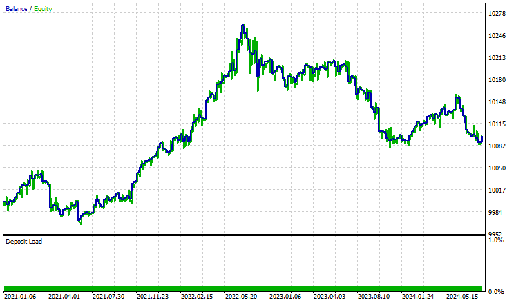
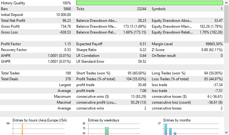
I ran a test on the Strategy Tester from 2021.01.01 to 2024.10.8 on a 4-Hour timeframe, Modelling was set to "Open prices only". Below is the outcome.

The EA did well, to say the least, providing 55% profitable trades which provided a total net profit of $96 USD. Not bad for a simple dataset, simple model, and a minimal trading volume set-up.

Final Thoughts

CatBoost and other Gradient Boosted Decision Trees are a go-to solution when you are working in a limited resource environment and looking for a model that "just works" without having to do a lot of the boring and sometimes unnecessary stuff that goes into feature engineering and model configuration we often face when working with numerous machine models.

Despite their simplicity and their minimal entry barrier, they are among the best and most effective AI models used in many real-world applications.

Best regards.

Track development of machine learning models and much more discussed in this article series on this GitHub repo.

Attachments Table

File name	File type	Description & Usage
Experts\CatBoost EA.mq5	Expert Advisor	Trading robot for loading the Catboost model in ONNX format and testing the trading strategy in MetaTrader 5.
Include\CatBoost.mqh	Include file	Contains the code for loading and deploying a CatBoost model.
Files\ CatBoost.EURUSD.OHLC.D1.onnx	ONNX model	Trained CatBoost model saved in ONNX format.
Scripts\CollectData.mq5	MQL5 script	A script for collecting the training data.
Jupyter Notebook\CatBoost-4-trading.ipynb	Python/Jupyter notebook	All the Python code discussed in this article can be found inside this notebook.

Sources & References

Attached files |

Download ZIP

Attachments.zip (40.07 KB)

Warning: All rights to these materials are reserved by MetaQuotes Ltd. Copying or reprinting of these materials in whole or in part is prohibited.

What is CatBoost?

How Does CatBoost Operate?

CatBoost vs XGBoost and LightGBM, A Detailed Comparison

Deploying a CatBoost Model

Training a CatBoost Model

Evaluating the Model

Saving the CatBoost Model to ONNX

Creating a CatBoost Expert Advisor (Trading Robot)

Final Thoughts

Other articles by this author