Data Science and Machine Learning (Part 25): Forex Timeseries Forecasting Using a Recurrent Neural Network (RNN)

Contents

• What are the Recurrent Neural Networks (RNNs)
• Understanding RNNs
• Mathematics behind a Recurrent Neural Network(RNN)
• Building a Recurrent Neural Network(RNN) Model in Python
• Creating Sequential Data
• Training the Simple RNN for a Regression Problem
• RNN Feature Importance
• Training the Simple RNN for a Classification Problem
• Saving the Recurrent Neural Network Model to ONNX
• Recurrent Neural Network(RNN) Expert Advisor
• Testing Recurrent Neural Network EA on the Strategy Tester
• Advantages of Using Simple RNN for Timeseries Forecasting
• Conclusion

What are the Recurrent Neural Networks (RNNs)

Recurrent Neural Networks (RNNs) are artificial neural networks designed to recognize patterns in sequences of data, such as time series, language, or video. Unlike traditional neural networks, which assume that inputs are independent of each other, RNNs can detect and understand patterns from a sequence of data (information).

Not to be confused with the terminologies throughout this article, When saying Recurrent Neural Network I refer to simple RNN as a model meanwhile, when I use Recurrent Neural Networks (RNNs) I refer to a family of recurrent neural network models such as simple RNN, Long Short Term Memory (LSTM) and Gated Recurrent Unit (GRU).

A basic understanding of Python, ONNX in MQL5, and Python machine learning is required to understand the contents of this article fully.

Understanding RNNs

RNNs have something called sequential memory, which refers to the concept of retaining and utilizing information from the previous time steps in a sequence to inform the processing of subsequent time steps.

Sequential memory is similar to the one in your human brain, It is the kind of memory that makes it easier for you to recognize patterns in sequences, such as when articulating for words to speak.

At the core of Recurrent Neural Networks(RNNs), there are feedforward neural networks interconnected in such a way that the next network has the information from the previous one, giving the simple RNN the ability to learn and understand the current information based on the prior ones.

To understand this better, let us look at an example where we want to teach the RNN model for a chatbot, we want our chatbot to understand the words and sentences from a user, suppose the sentence received is; What time is it?

The words will be split into their respective Timesteps and fed into the RNN one after the other, as seen in the image below.

Looking at the last node in the network, you may have noticed an odd arrangement of colors representing the information from the previous networks and the current one. Looking at the colors the information from the network at time t=0 and time t=1 is too tiny(almost nonexistent) in this last node of the RNN.

As the RNN processes more steps it has trouble retaining information from the previous steps. As seen in the image above, the words what and time are almost nonexistent in the final node of the network.

This is what we call short-term memory. It is caused by many factors backpropagation being one of the major.

Recurrent Neural Networks(RNNs) have their own backpropagation process known as backpropagation through time. During backpropagation, the gradient values exponentially shrink as the network propagates through each time step backward. Gradients are used to make adjustments to neural network parameters(weights and bias), this adjustment is what allows the neural network to learn. Small gradients mean smaller adjustments. Since early layers receive small gradients, this causes them not to learn as effectively as they should. This is referred to as the vanishing gradients problem.

Because of the vanishing gradient issue, the simple RNN doesn't learn long-range dependencies across time steps. In the image example above, there is a huge possibility that words such as what and time are not considered at all when our chatbot RNN model tries to understand an example sentence from a user. The network has to make its best guess with half a sentence with three words only; is it ?, This makes the RNN less effective as its memory is too short to understand long Time series data which is often found in real-world applications.

To mitigate short-term memory two specialized Recurrent Neural Networks, Long Short Term Memory (LSTM) and Gated Recurrent Unit (GRU) were introduced.

Both LSTM and GRU work similarly in many ways to RNN, but they are capable of understanding long-term dependencies using the mechanism called gates. We will discuss them in detail in the next article stay tuned.

Mathematics behind a Recurrent Neural Network(RNN)

Unlike Feed-forward neural networks, RNNs have connections that form cycles, allowing information to persist. The simplistic image below shows what a RNN unit/cell looks like when dissected.

Where:

 is the input at time t.

 is the hidden state at time t.

Hidden State

Denoted as , This is a vector that stores information from the previous time steps. It acts as the memory of the network allowing it to capture temporal dependencies and patterns in the input data over time.

Roles of hidden state to the network

The hidden state serves several crucial functions in a RNN such as;

• It retains information from previous inputs, This enables the network to learn from the entire sequence.
• It provides context for the current input, This allows the network to make informed predictions based on past data.
• It forms the basis for the recurrent connections within the network, This allows the hidden layer to influence itself across different time steps.

Understanding the mathematics behind RNN isn't as important as knowing the how, where, and when to use them, Feel free to jump to the next section of this article if you wish to.

Mathematical Formula

The hidden state at time step   is computed using the input at time step     , the hidden state from the previous time step   and corresponding weight matrices and biases. The formula is as follows;

Where:

 is the weight matrix for the input to the hidden state.

 is the weight matrix for the hidden state to the hidden state.

 is the bias term for the hidden state.

σ is the activation function (e.g., tanh or ReLU).

Output Layer

The output at time step  is computed from the hidden state at time step  .

 

Where

 is the output at time step  .

 is the weight matrix from hidden state to the output.

 bias of the output layer.

Loss Calculation

Assuming a loss function  (This can be any loss function, eg. Mean Squared Error for regression or Cross-Entropy for classification).

The total loss over all time steps is;

Backpropagation Through Time (BPTT)

To update both weights and bias, we need to compute the gradients of the loss with respect to each weight and bias respectively then use the obtained gradients to make updates. This involves the steps outlined below.

Step	For weights	For Bias
Computing gradient of the output layer	with respect to weights: Where   is the gradient of the loss wrt the output.	with respect to bias: Since output bias   affects outputs directly we have; Therefore.
Computing gradients of the hidden state with respect to weights and bias	The gradient of the loss wrt the hidden state involves both the direct contribution from the current time step and the indirect contribution through the subsequent time steps. Gradient of the hidden state wrt previous time step. Gradient of the hidden state activation. Gradient of the hidden layer weights. The total gradient is the sum of gradients over all time steps.	The gradient of the loss with respect to the hidden bias  is given by the sum of the gradients of the loss with respect to the hidden state  over all time steps. Since the hidden bias  affects the hidden state through the activation function, we have;   Using the chain rule and noting that; Where,   is the derivative of the activation function. Therefore:   The total gradient for the hidden bias is the sum of the gradients over all time steps.
Updating weights and bias. Using the gradients computed above, we can update the weights using gradient descent or any of its variants (e.g. Adam), read more.

Despite simple RNN(RNN) not having the ability to learn well long timeseries data, they are still good at predicting future values using information from the past not too long ago. We can build a simple RNN to help us in making trading decisions.

Building a Recurrent Neural Network(RNN) Model in Python

Building and Compiling a RNN model in Python is straightforward and takes a few lines of code using the Keras library.

Python

import tensorflow as tf
from tensorflow.keras.models import Sequential #import sequential neural network layer
from sklearn.preprocessing import StandardScaler
from tensorflow.keras.layers import SimpleRNN, Dense, Input
from keras.callbacks import EarlyStopping
from sklearn.preprocessing import MinMaxScaler
from keras.optimizers import Adam

reg_model = Sequential()

reg_model.add(Input(shape=(time_step, x_train.shape[1]))) # input layer
reg_model.add(SimpleRNN(50, activation='sigmoid')) #first hidden layer
reg_model.add(Dense(50, activation='sigmoid')) #second hidden layer
reg_model.add(Dense(units=1, activation='relu'))  # final layer 

adam_optimizer = Adam(learning_rate = 0.001)

reg_model.compile(optimizer=adam_optimizer, loss='mean_squared_error') # Compile the model
reg_model.summary()

The above code is for a regression recurrent neural network that's why we have 1 node in the output layer and a Relu activation function in the final layer, there is a reason for this. As discussed in the article Feed Forward Neural Networks Demystified.

Using the data we collected in the previous article Forex Timeseries Forecasting using regular ML models(a must-read), we want to see how we can use RNNs models as they are capable of understanding Timeseries data to aid us in what they are good at.

In the end, we will assess the performance of RNNs in contrast to LightGBM built in the prior article, on the same data. Hopefully, this will help solidify your understanding of Timeseries forecasting in general.

Creating Sequential Data

In our dataset we have 28 columns, all engineered for a non-timeseries model.

However, this data we collected and engineered has a lot of lagged variables which were handy for the non-timeseries model to detect time-dependent patterns. As we know RNNs can understand patterns within the given time-steps.

We do not need these lagged values for now, we have to drop them.

Python

lagged_columns = [col for col in data.columns if "lag" in col.lower()] #let us obtain all the columns with the name lag

print("lagged columns: ",lagged_columns)

data = data.drop(columns=lagged_columns) #drop them

Outputs

lagged columns:  ['OPEN_LAG1', 'HIGH_LAG1', 'LOW_LAG1', 'CLOSE_LAG1', 'OPEN_LAG2', 'HIGH_LAG2', 'LOW_LAG2', 'CLOSE_LAG2', 'OPEN_LAG3', 'HIGH_LAG3', 'LOW_LAG3', 'CLOSE_LAG3', 'DIFF_LAG1_OPEN', 'DIFF_LAG1_HIGH', 'DIFF_LAG1_LOW', 'DIFF_LAG1_CL

The new data has now 12 columns.

We can split 70% of the data into training while the rest 30% for testing. If you are using train_test_split from Scikit-Learn be sure to set shuffle=False. This will make the function split the original while preserving the order of information present.

Remember! This is Timeseries forecasting.

# Split the data

X = data.drop(columns=["TARGET_CLOSE","TARGET_OPEN"]) #dropping the target variables
Y = data["TARGET_CLOSE"]

test_size = 0.3 #70% of the data should be used for training purpose while the rest 30% should be used for testing

x_train, x_test, y_train, y_test = train_test_split(X, Y, shuffle=False, test_size = test_size) # this is timeseries data so we don't shuffle

print(f"x_train {x_train.shape}\nx_test {x_test.shape}\ny_train{y_train.shape}\ny_test{y_test.shape}")

After also dropping the two target variables, our data now remains with 10 features. We need to convert these 10 features into sequential data that RNNs can digest.

def create_sequences(X, Y, time_step):
    if len(X) != len(Y):
        raise ValueError("X and y must have the same length")
    
    X = np.array(X)
    Y = np.array(Y)
    
    Xs, Ys = [], []
    
    for i in range(X.shape[0] - time_step):
        Xs.append(X[i:(i + time_step), :])  # Include all features with slicing
        Ys.append(Y[i + time_step])
        
    return np.array(Xs), np.array(Ys)

The above function generates a sequence from given x and y arrays for a specified time step. To understand how this function works, read the following example;

Suppose we have a dataset with 10 samples and 2 features, and we want to create sequences with a time step of 3.

X which is a matrix of shape (10, 2). Y which is a vector of length 10.
The function will create sequences as follows
For i=0: Xs gets [0:3, :] X[0:3, :], and Ys gets Y[3]. For i=1: Xs gets 𝑋[1:4, :] X[1:4, :], and Ys gets Y[4].

And so on, until i=6.

The resulting Xs will have a shape of (7, 3, 2), and Ys will have a length of 7

After standardizing the independent variables that we have split up, we can then apply the function create_sequences to generate sequential information.

time_step = 7 # we consider the past 7 days

from sklearn.preprocessing import StandardScaler

scaler = StandardScaler()

x_train = scaler.fit_transform(x_train)
x_test = scaler.transform(x_test)

x_train_seq, y_train_seq = create_sequences(x_train, y_train, time_step)
x_test_seq, y_test_seq = create_sequences(x_test, y_test, time_step)

print(f"Sequential data\n\nx_train {x_train_seq.shape}\nx_test {x_test_seq.shape}\ny_train{y_train_seq.shape}\ny_test{y_test_seq.shape}")

Outputs

Sequential data

x_train (693, 7, 10)
x_test (293, 7, 10)
y_train(693,)
y_test(293,)

The time step value of 7 ensures that at each instance the RNN is plugged with the information from the past 7 days, considering that we collected all information present in the dataset from the daily timeframe. This is similar to manually obtaining lags for the previous 7 days from the current bar, something we did in the previous article of this series.

Training the Simple RNN for a Regression Problem

early_stopping = EarlyStopping(monitor='val_loss', patience=5, restore_best_weights=True)

history = reg_model.fit(x_train_seq, y_train_seq, epochs=100, batch_size=64, verbose=1, validation_data=(x_test_seq, y_test_seq), callbacks=[early_stopping])

Outputs

Epoch 95/100
11/11 ━━━━━━━━━━━━━━━━━━━━ 0s 8ms/step - loss: 6.4504e-05 - val_loss: 4.4433e-05
Epoch 96/100
11/11 ━━━━━━━━━━━━━━━━━━━━ 0s 8ms/step - loss: 6.4380e-05 - val_loss: 4.4408e-05
Epoch 97/100
11/11 ━━━━━━━━━━━━━━━━━━━━ 0s 8ms/step - loss: 6.4259e-05 - val_loss: 4.4386e-05
Epoch 98/100
11/11 ━━━━━━━━━━━━━━━━━━━━ 0s 8ms/step - loss: 6.4140e-05 - val_loss: 4.4365e-05
Epoch 99/100
11/11 ━━━━━━━━━━━━━━━━━━━━ 0s 7ms/step - loss: 6.4024e-05 - val_loss: 4.4346e-05
Epoch 100/100
11/11 ━━━━━━━━━━━━━━━━━━━━ 0s 7ms/step - loss: 6.3910e-05 - val_loss: 4.4329e-05

After measuring the performance of the testing sample.

Python

from sklearn.metrics import r2_score

y_pred = reg_model.predict(x_test_seq) # Make predictions on the test set

# Plot the actual vs predicted values
plt.figure(figsize=(12, 6))
plt.plot(y_test_seq, label='Actual Values')
plt.plot(y_pred, label='Predicted Values')
plt.xlabel('Samples')
plt.ylabel('TARGET_CLOSE')
plt.title('Actual vs Predicted Values')
plt.legend()
plt.show()

print("RNN accuracy =",r2_score(y_test_seq, y_pred))

The model was 78% percent accurate.

If you remember from the previous article, the LightGBM model was 86.76% accurate on a regression problem, at this point a non-timeseries model has outperformed a Timeseries one.  

Feature Importance

I ran a test to check how variables affect the RNN model decision-making process using SHAP.

import shap

# Wrap the model prediction for KernelExplainer
def rnn_predict(data):
    data = data.reshape((data.shape[0], time_step, x_train.shape[1]))
    return reg_model.predict(data).flatten()

# Use SHAP to explain the model
sampled_idx = np.random.choice(len(x_train_seq), size=100, replace=False)
explainer = shap.KernelExplainer(rnn_predict, x_train_seq[sampled_idx].reshape(100, -1))
shap_values = explainer.shap_values(x_test_seq[:100].reshape(100, -1), nsamples=100)

I ran code to draw a plot for feature importance.

# Update feature names for SHAP
feature_names = [f'{original_feat}_t{t}' for t in range(time_step) for original_feat in X.columns]

# Plot the SHAP values
shap.summary_plot(shap_values, x_test_seq[:100].reshape(100, -1), feature_names=feature_names, max_display=len(feature_names), show=False)

# Adjust layout and set figure size
plt.subplots_adjust(left=0.12, bottom=0.1, right=0.9, top=0.9)  
plt.gcf().set_size_inches(7.5, 14) 
plt.tight_layout()

plt.savefig("regressor-rnn feature-importance.png")
plt.show()

Below was the outcome.

The most impactful variables are the ones with recent information, meanwhile the less impactful variables are ones with the oldest information.

This is just like saying the most recent word spoken in a sentence carries the most meaning for the whole sentence.

This may be true for a machine learning model despite not making much sense to us human beings.

As said in the previous article, we can not trust the feature importance plot alone, considering I have used KernelExplainer instead of the recommended DeepExplainer which I experienced lots of errors getting the method it to work.

As said in the previous article having a regression model to guess the next close or open price isn't as practical as having a classifier that tells us where it thinks the market is heading in the next bar. Let us make a RNN classifier model to help us with that task.

Training the Simple RNN for a Classification Problem

We can follow a similar process we did while coding for a regressor with a few changes; First of all, we need to create the target variable for the classification problem.

Python

Y = []
target_open = data["TARGET_OPEN"]
target_close = data["TARGET_CLOSE"]

for i in range(len(target_open)):
    if target_close[i] > target_open[i]: # if the candle closed above where it opened thats a buy signal
        Y.append(1)
    else: #otherwise it is a sell signal
        Y.append(0)
        
Y = np.array(Y) #converting this array to NumPy


classes_in_y = np.unique(Y) # obtaining classes present in the target variable for the sake of setting the number of outputs in the RNN

Then we must one-hot-encode the target variable shortly after the sequence is created as discussed during the making of a regression model.

from tensorflow.keras.utils import to_categorical

y_train_encoded = to_categorical(y_train_seq)
y_test_encoded = to_categorical(y_test_seq)

print(f"One hot encoded\n\ny_train {y_train_encoded.shape}\ny_test {y_test_encoded.shape}")

Outputs

One hot encoded

y_train (693, 2)
y_test (293, 2)

Finally, we can build the classifier RNN model and train it.

cls_model = Sequential()

cls_model.add(Input(shape=(time_step, x_train.shape[1]))) # input layer
cls_model.add(SimpleRNN(50, activation='relu'))
cls_model.add(Dense(50, activation='relu'))
cls_model.add(Dense(units=len(classes_in_y), activation='sigmoid', name='outputs')) 


adam_optimizer = Adam(learning_rate = 0.001)

cls_model.compile(optimizer=adam_optimizer, loss='binary_crossentropy') # Compile the model
cls_model.summary()


early_stopping = EarlyStopping(monitor='val_loss', patience=5, restore_best_weights=True)

history = cls_model.fit(x_train_seq, y_train_encoded, epochs=100, batch_size=64, verbose=1, validation_data=(x_test_seq, y_test_encoded), callbacks=[early_stopping])

For the classifier RNN model, I used sigmoid for the final layer in the network. The number of neurons(units) in the final layer must match the number of classes present in the target variable(Y), in this case we we are going to have two units.

Model: "sequential_1"
┏━━━━━━━━━━━━━━━━━━━━━━━━━━━━━━━━━┳━━━━━━━━━━━━━━━━━━━━━━━━┳━━━━━━━━━━━━━━━┓
┃ Layer (type)                    ┃ Output Shape           ┃       Param # ┃
┡━━━━━━━━━━━━━━━━━━━━━━━━━━━━━━━━━╇━━━━━━━━━━━━━━━━━━━━━━━━╇━━━━━━━━━━━━━━━┩
│ simple_rnn_1 (SimpleRNN)        │ (None, 50)             │         3,050 │
├─────────────────────────────────┼────────────────────────┼───────────────┤
│ dense_2 (Dense)                 │ (None, 50)             │         2,550 │
├─────────────────────────────────┼────────────────────────┼───────────────┤
│ outputs (Dense)                 │ (None, 2)              │           102 │
└─────────────────────────────────┴────────────────────────┴───────────────┘

6 epochs were enough for the RNN classifier model to converge during training.

Epoch 1/100
11/11 ━━━━━━━━━━━━━━━━━━━━ 2s 36ms/step - loss: 0.7242 - val_loss: 0.6872
Epoch 2/100
11/11 ━━━━━━━━━━━━━━━━━━━━ 0s 9ms/step - loss: 0.6883 - val_loss: 0.6891
Epoch 3/100
11/11 ━━━━━━━━━━━━━━━━━━━━ 0s 8ms/step - loss: 0.6817 - val_loss: 0.6909
Epoch 4/100
11/11 ━━━━━━━━━━━━━━━━━━━━ 0s 8ms/step - loss: 0.6780 - val_loss: 0.6940
Epoch 5/100
11/11 ━━━━━━━━━━━━━━━━━━━━ 0s 8ms/step - loss: 0.6743 - val_loss: 0.6974
Epoch 6/100
11/11 ━━━━━━━━━━━━━━━━━━━━ 0s 8ms/step - loss: 0.6707 - val_loss: 0.6998

Despite having a lower accuracy on the regression task compared to the accuracy provided by the LightGBM regressor, The RNN classifier model was 3% more accurate than the LightGBM classifier.

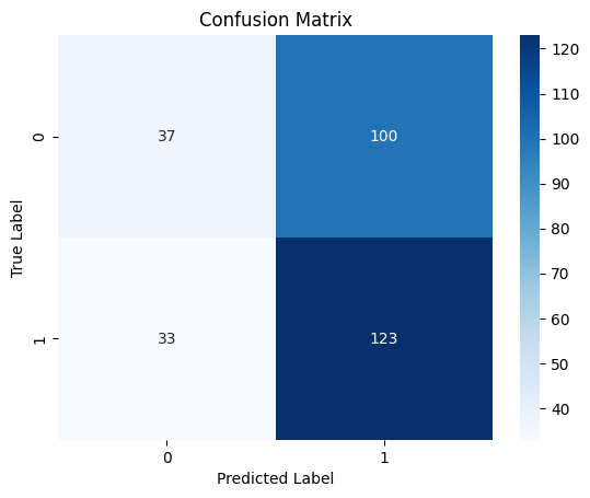
10/10 ━━━━━━━━━━━━━━━━━━━━ 0s 19ms/step
Classification Report
               precision    recall  f1-score   support

           0       0.53      0.27      0.36       137
           1       0.55      0.79      0.65       156

    accuracy                           0.55       293
   macro avg       0.54      0.53      0.50       293
weighted avg       0.54      0.55      0.51       293

Confusion matrix heatmap

Saving the Recurrent Neural Network Model to ONNX

Now that we have a classifier RNN model, we can save it to the ONNX format that is understood by MetaTrader 5.

Unlike Scikit-learn models, saving Keras deep learning models like RNNs isn't straighforward-easy. Pipelines aren't an easy solution either for RNNs.

As discussed in the article Overcoming ONNX challenges, we can either scale the data in MQL5 shortly after collecting or we can save the scaler we have in Python and load it in mql5 using the preprocessing library for MQL5.

Saving the Model

import tf2onnx

# Convert the Keras model to ONNX
spec = (tf.TensorSpec((None, time_step, x_train.shape[1]), tf.float16, name="input"),)
cls_model.output_names=['output']

onnx_model, _ = tf2onnx.convert.from_keras(cls_model, input_signature=spec, opset=13)

# Save the ONNX model to a file
with open("rnn.EURUSD.D1.onnx", "wb") as f:
    f.write(onnx_model.SerializeToString())

Saving the Standardization Scaler parameters

# Save the mean and scale parameters to binary files

scaler.mean_.tofile("standard_scaler_mean.bin")
scaler.scale_.tofile("standard_scaler_scale.bin")

By saving mean and standard deviation which are the main components of the Standard scaler, we can be confident that we have successfully saved the Standard scaler. 

Recurrent Neural Network(RNN) Expert Advisor

Inside our EA, the first thing we have to do is to add both the RNN model that is in ONNX format and the Standard Scaler binary files as resource files to our EA.

MQL5 | RNN timeseries forecasting.mq5

#resource "\\Files\\rnn.EURUSD.D1.onnx" as uchar onnx_model[]; //rnn model in onnx format
#resource "\\Files\\standard_scaler_mean.bin" as double standardization_mean[];
#resource "\\Files\\standard_scaler_scale.bin" as double standardization_std[];

We can then load the libraries for both loading RNN model in ONNX format and the Standard scaler.

MQL5

#include <MALE5\Recurrent Neural Networks(RNNs)\RNN.mqh>
CRNN rnn;

#include <MALE5\preprocessing.mqh>
StandardizationScaler *scaler; 

Inside the OnInit function.

vector classes_in_data_ = {0,1}; //we have to assign the classes manually | it is very important that their order is preserved as they can be seen in python code, HINT: They are usually in ascending order
//+------------------------------------------------------------------+
//| Expert initialization function                                   |
//+------------------------------------------------------------------+
int OnInit()
  {
  
//--- Initialize ONNX model
   
   if (!rnn.Init(onnx_model))
     return INIT_FAILED;
   
//--- Initializing the scaler with values loaded from binary files 

   scaler = new StandardizationScaler(standardization_mean, standardization_std);
   
//--- Initializing the CTrade library for executing trades

   m_trade.SetExpertMagicNumber(magic_number);
   m_trade.SetDeviationInPoints(slippage);
   m_trade.SetMarginMode();
   m_trade.SetTypeFillingBySymbol(Symbol());
           
   lotsize = SymbolInfoDouble(Symbol(), SYMBOL_VOLUME_MIN);
   
//--- Initializing the indicators

   ma_handle = iMA(Symbol(),timeframe,30,0,MODE_SMA,PRICE_WEIGHTED); //The Moving averaege for 30 days
   stddev_handle = iStdDev(Symbol(), timeframe, 7,0,MODE_SMA,PRICE_WEIGHTED); //The standard deviation for 7 days
   

   return(INIT_SUCCEEDED);
  }

Before we can deploy the model for live trading inside the OnTick function, we have to collect data similarly to how we collected the training data But, this time we have to avoid the features we dropped during training.

Remember! We trained the model with 10 features(independent variables) only.

Let us make the function GetInputData to collect those 10 independent variables only.

matrix GetInputData(int bars, int start_bar=1)
 {
   vector open(bars), 
          high(bars),
          low(bars), 
          close(bars), 
          ma(bars), 
          stddev(bars), 
          dayofmonth(bars), 
          dayofweek(bars), 
          dayofyear(bars), 
          month(bars);

//--- Getting OHLC values
   
   open.CopyRates(Symbol(), timeframe, COPY_RATES_OPEN, start_bar, bars);
   high.CopyRates(Symbol(), timeframe, COPY_RATES_HIGH, start_bar, bars);
   low.CopyRates(Symbol(), timeframe, COPY_RATES_LOW, start_bar, bars);
   close.CopyRates(Symbol(), timeframe, COPY_RATES_CLOSE, start_bar, bars);
   
   vector time_vector;
   time_vector.CopyRates(Symbol(), timeframe, COPY_RATES_TIME, start_bar, bars);
   
//---

   
   ma.CopyIndicatorBuffer(ma_handle, 0, start_bar, bars); //getting moving avg values 
   stddev.CopyIndicatorBuffer(stddev_handle, 0, start_bar, bars); //getting standard deviation values
   
   string time = "";
   for (int i=0; i<bars; i++) //Extracting time features 
     {
       time = (string)datetime(time_vector[i]); //converting the data from seconds to date then to string
       TimeToStruct((datetime)StringToTime(time), date_time_struct); //convering the string time to date then assigning them to a structure
       
       dayofmonth[i] = date_time_struct.day;
       dayofweek[i] = date_time_struct.day_of_week;
       dayofyear[i] = date_time_struct.day_of_year;
       month[i] = date_time_struct.mon;
     }
   
   matrix data(bars, 10); //we have 10 inputs from rnn | this value is fixed
   
//--- adding the features into a data matrix
   
   data.Col(open, 0);
   data.Col(high, 1);
   data.Col(low, 2);
   data.Col(close, 3);
   data.Col(ma, 4);
   data.Col(stddev, 5);
   data.Col(dayofmonth, 6);
   data.Col(dayofweek, 7);
   data.Col(dayofyear, 8);
   data.Col(month, 9);
   
   return data;
 }

Finally, we can deploy the RNN model to give us trading signals for our simple strategy.

void OnTick()
  {
//---
   
   if (NewBar()) //Trade at the opening of a new candle
    {
      matrix input_data_matrix = GetInputData(rnn_time_step);
      input_data_matrix = scaler.transform(input_data_matrix); //applying StandardSCaler to the input data
      
      int signal = rnn.predict_bin(input_data_matrix, classes_in_data_); //getting trade signal from the RNN model
     
      Comment("Signal==",signal);
     
   //---
     
      MqlTick ticks;
      SymbolInfoTick(Symbol(), ticks);
      
      if (signal==1) //if the signal is bullish
       {
          if (!PosExists(POSITION_TYPE_BUY)) //There are no buy positions
           {
             if (!m_trade.Buy(lotsize, Symbol(), ticks.ask, ticks.bid-stoploss*Point(), ticks.ask+takeprofit*Point())) //Open a buy trade
               printf("Failed to open a buy position err=%d",GetLastError());
           }
       }
      else if (signal==0) //Bearish signal
        {
          if (!PosExists(POSITION_TYPE_SELL)) //There are no Sell positions
            if (!m_trade.Sell(lotsize, Symbol(), ticks.bid, ticks.ask+stoploss*Point(), ticks.bid-takeprofit*Point())) //open a sell trade
               printf("Failed to open a sell position err=%d",GetLastError());
        }
      else //There was an error
        return;
    }
  }

Testing Recurrent Neural Network EA on the Strategy Tester

With a trading strategy in place, Let us run tests in the strategy tester. I am using the same Stop loss and Take profit values we used for the LightGBM model, including the tester settings.

input group "rnn";
input uint rnn_time_step = 7; 
//this value must be the same as the one used during training in a python script

input ENUM_TIMEFRAMES timeframe = PERIOD_D1;
input int magic_number = 1945;
input int slippage = 50;
input int stoploss = 500;
input int takeprofit = 700;

Strategy tester settings:

The EA was 44.56% profitable in the 561 trades it took.

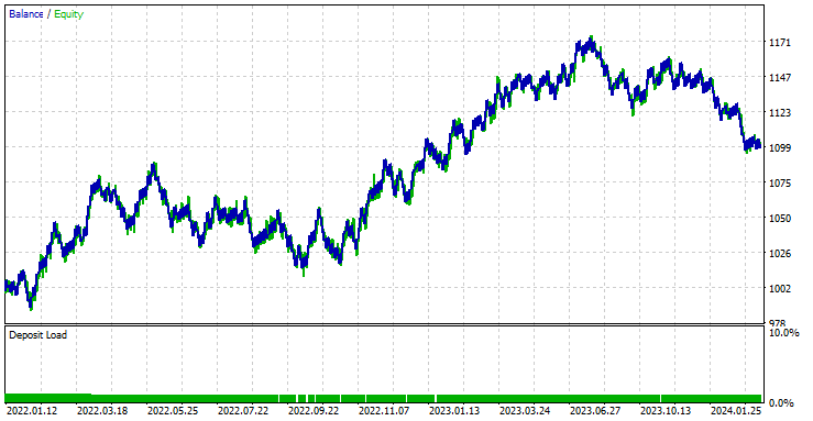
With the current Stop loss and Take profit values it is fair to say the LightGBM model outperformed a simple RNN model for Timeseries forecasting as it made a net profit of 572 $ compared to RNN which made a net profit of 100 $.

I ran an optimization to find the best Stop loss and Take profit values, and one of the best values was a Stop Loss of 1000 points and a Take profit of 700 points.

Advantages of Using Simple RNN for Timeseries Forecasting

• They Can handle Sequential data
  Simple RNNs are designed to handle sequence data and are well-suited for tasks where the order of data points matters, such as time series prediction, language modeling, and speech recognition.
  
  
• They share parameters across different time steps
  This helps in learning temporal patterns effectively. This parameter sharing makes the model efficient in terms of the number of parameters, especially when compared to models that treat each time step independently.
  
  
• They are capable of capturing Temporal Dependencies
  They can capture dependencies over time, which is essential for understanding context in sequential data. They can model short-term temporal dependencies effectively.
  
  
• Flexible in Sequence Length
  Simple RNNs can handle variable-length sequences, making them flexible for different types of sequential data inputs.
  
  
• Simple to use and Implement
  The architecture of a simple RNN is relatively easy to implement. This simplicity can be beneficial for understanding the fundamental concepts of sequence modeling.

Final Thoughts

This article gives you an in-depth understanding of a simple Recurrent Neural Network and how it can be deployed in the MQL5 programming language. Throughout the article, I have often compared the results of the RNN model to the LightGBM model we built in the previous article of this series only for the sake of sharpening your understanding of Timeseries forecasting using Timeseries and non-timeseries-based models.

The comparison is unfair in many terms considering these two models are very different in structure and how they make predictions, Any conclusion drawn in the article by me or by a reader's mind should be disregarded.

it is worth mentioning that the RNN model was not fed with similar data compared to the LightGBM model, In this article we removed some lags which were differentiated values between OHLC price values (DIFF_LAG1_OPEN, DIFF_LAG1_HIGH, DIFF_LAG1_LOW and, DIFF_LAG1_CLOSE).

We could have non-lagged values for this that RNN will auto-detect their lags but we chose to not include them at all since they weren't present in the dataset. 

Best regards.

Track development of machine learning models and much more discussed in this article series on this GitHub repo.

Attachments Table

File name	File type	Description & Usage
RNN timeseries forecasting.mq5	Expert Advisor	Trading robot for loading the RNN ONNX model and testing the final trading strategy in MetaTrader 5.
rnn.EURUSD.D1.onnx	ONNX	RNN model in ONNX format.
standard_scaler_mean.bin standard_scaler_scale.bin	Binary files	Binary files for the Standardization scaler
preprocessing.mqh	An Include file	A library which consists of the Standardization Scaler
RNN.mqh	An Include file	A library for loading and deploying ONNX model
rnns-for-forex-forecasting-tutorial.ipynb	Python Script/Jupyter Notebook	Consists all the python code discussed in this article

Sources & References

• Illustrated Guide to Recurrent Neural Networks: Understanding the Intuition(https://www.youtube.com/watch?v=LHXXI4-IEns)
• Recurrent Neural Networks - Ep. 9 (Deep Learning SIMPLIFIED) (https://youtu.be/_aCuOwF1ZjU)
• Recurrent Neural networks(https://stanford.edu/~shervine/teaching/cs-230/cheatsheet-recurrent-neural-networks#)