
Data Science and ML (Part 26): The Ultimate Battle in Time Series Forecasting — LSTM vs GRU Neural Networks

Contents
- What is a Long Short-Term Memory (LSTM) neural network?
- Mathematics behind the Long-Short-Term Memory(LSTM) network
- What is a gated recurrent unit(GRU) neural network?
- Mathematics behind the gated recurrent unit (GRU) network
- Building the parent class for LSTM and GRU networks
- LSTM and GRU neural network child classes
- Training both models
- Checking feature importance for both models
- LSTM versus GRU classifiers on the strategy tester
- The differences between LSTM and GRU neural network models
- Conclusion
What is a Long Short-Term Memory (LSTM) Neural Network?
Long Short-Term Memory(LSTM), is a type of recurrent neural network designed for sequence tasks, excelling in capturing and utilizing long-term dependencies in data. Unlike vanilla Recurrent Neural Networks(simple RNNs) discussed in the previous article of this series (a must-read). Which can't capture long-term dependencies in the data.
LSTMs were introduced to fix the short-term memory which is prevalent in simple RNNs.
The Problem with Simple Recurrent Neural Networks
Simple Recurrent Neural Networks (RNNs) are designed to handle sequential data by using their internal hidden state (memory) to capture information about previous inputs in the sequence. Despite their conceptual simplicity and initial success in modeling sequential data, they have several limitations.
One significant issue is the vanishing gradient problem. During backpropagation, gradients are used to update the weights of the network. In simple RNNs, these gradients can diminish exponentially as they are propagated backward through time, especially for long sequences. This results in the network's inability to learn long-term dependencies, as the gradients become too small to make effective updates to the weights, making it difficult for simple RNNs to capture patterns that span over many time steps.
Another challenge is the exploding gradient problem, which is the opposite of the vanishing gradient problem. In this case, gradients grow exponentially during backpropagation. This can cause numerical instability and make the training process very challenging. Although less common than vanishing gradients, exploding gradients can lead to wildly large updates to the network's weights, effectively causing the learning process to fail.
Simple RNNs are also difficult to train due to their susceptibility to both vanishing and exploding gradient problems, which can make the training process inefficient and slow. Training simple RNNs can be more computationally expensive and may require careful tuning of hyperparameters.
Furthermore, simple RNNs are unable to handle complex temporal dependencies in data. Due to their limited memory capacity, they often struggle to understand and capture complex sequential patterns.
For tasks that involve an understanding of long-range dependencies in the data, simple RNNs may fail to capture the necessary context, leading to suboptimal performance.
Mathematics Behind the Long Short-Term Memory(LSTM) Network
To understand the nitty-gritty behind LSTM, firstly let us look at the LSTM cell.

01: Forget Gate
Given by the equation.
![]()
A sigmoid function ![]() takes as input the previous hidden state
takes as input the previous hidden state ![]() and the current input
and the current input ![]() . The output
. The output ![]() is a value between 0 and 1, indicating how much of each component in
is a value between 0 and 1, indicating how much of each component in ![]() (previous cell state) should be retained.
(previous cell state) should be retained.
![]() - weight of the forget gate.
- weight of the forget gate.
![]() - bias of the forget gate.
- bias of the forget gate.
The forget gate determines which information from the previous cell state should be carried forward. It outputs a number between 0 and 1 for each number in the cell state ![]() , where 0 means completely forget and 1 means completely retain.
, where 0 means completely forget and 1 means completely retain.
02: Input Gate
Given by the formula.
![]()
A sigmoid function ![]() determines which values to update. This gate controls the input of new data into the memory cell.
determines which values to update. This gate controls the input of new data into the memory cell.
![]() - weight input gate.
- weight input gate.
![]() - bias input gate.
- bias input gate.
This gate decides which values from the new input ![]() are used to update the cell state. It regulates the flow of new information into the cell.
are used to update the cell state. It regulates the flow of new information into the cell.
03: Candidate Memory Cell
Given by the equation.
![]()
A tanh function generates potential new information that could be stored in the cell state.
![]() - Weight of the candidate memory cell.
- Weight of the candidate memory cell.
![]() - Bias of the candidate memory cell.
- Bias of the candidate memory cell.
This component generates the new candidate values that can be added to the cell state. It uses the tanh activation function to ensure the values are between -1 and 1.
04: Cell State Update
Given by the equation.
![]()
The previous cell state ![]() is multiplied by
is multiplied by ![]() (forget gate output) to discard unimportant information. Then,
(forget gate output) to discard unimportant information. Then, ![]() (input gate output) is multiplied by
(input gate output) is multiplied by ![]() (candidate cell state), and the results are summed to form the new cell state
(candidate cell state), and the results are summed to form the new cell state ![]() .
.
The cell state is updated by combining the old cell state and the candidate values. The forget gate output controls the previous cell state contribution, and the input gate output controls the new candidate values' contribution.
05: Output Gate
Given by the equation.
![]()
A sigmoid function determines which parts of the cell state to output. This gate controls the output of information from the memory cell.
![]() - Weight of the output layer
- Weight of the output layer
![]() - Bias of the output layer
- Bias of the output layer
This gate determines the final output for the current cell state. It decides which parts of the cell state should be output based on the input ![]() and the previous hidden state
and the previous hidden state ![]() .
.
06: Hidden State Update
Given by the equation.
![]()
The new hidden state ![]() is obtained by multiplying the output gate
is obtained by multiplying the output gate ![]() with the tanh of the updated cell state
with the tanh of the updated cell state ![]() .
.
The hidden state is updated based on the cell state and the output gate's decision. It is used as the output for the current time step and as an input for the next time step
What is a Gated Recurrent Unit(GRU) Neural Network?
The Gated Recurrent Unit (GRU) is a type of Recurrent Neural Network (RNN) that, in certain cases, has advantages over long short-term memory (LSTM). GRU uses less memory and is faster than LSTM, however, LSTM is more accurate when using datasets with longer sequences.
LSTMs and GRUs were introduced to mitigate short-term memory prevalent in simple recurrent neural networks. Both have long-term memory enabled by using the gates in their cells.
Despite working similarly to simple RNNs in many ways, LSTMs and GRUs address the vanishing gradient problem from which simple recurrent neural networks suffer.
Mathematics Behind the Gated Recurrent Unit (GRU) Network
The image below illustrates how the GRU cell looks when dissected.

01: The Update Gate
Given by the formula.
![]()
This gate determines how much of the previous hidden state ![]() should be retained and how much of the candidate hidden state
should be retained and how much of the candidate hidden state ![]() should be used to update the hidden state.
should be used to update the hidden state.
The update gate controls how much of the previous hidden state ![]() should be carried forward to the next time step. It effectively decides the balance between keeping the old information and incorporating new information.
should be carried forward to the next time step. It effectively decides the balance between keeping the old information and incorporating new information.
02: Reset Gate
Given by the formula.
![]()
The sigmoid function ![]() in this gate, determines which parts of the previous hidden state should be reset before combining with the current input to create the candidate activation.
in this gate, determines which parts of the previous hidden state should be reset before combining with the current input to create the candidate activation.
03: Candidate Activation
Given by the formula.
![]()
The candidate activation is computed using the current input ![]() and the reset hidden state
and the reset hidden state ![]() .
.
This component generates new potential values for the hidden state that can be incorporated based on the update gate's decision.
04: Hidden State Update
Given by the formula.
![]()
The update gate output ![]() controls how much of the candidate hidden state
controls how much of the candidate hidden state ![]() is used to form the new hidden state
is used to form the new hidden state ![]() .
.
The hidden state is updated by combining the previous hidden state and the candidate hidden state. The update gate ![]() controls this combination, ensuring that the relevant information from the past is retained while incorporating new information.
controls this combination, ensuring that the relevant information from the past is retained while incorporating new information.
Building the Parent Class for LSTM and GRU Networks
Since LSTM and GRU work similarly in many ways and they take the same parameters, it might be a good idea to have a base(parent) class for the functions necessary for building, compiling, optimizing, checking feature importance, and saving the models. This class will be inherited in the subsequent LSTM and GRU child classes.
import tensorflow as tf
from tensorflow.keras.models import Sequential
from tensorflow.keras.layers import LSTM, GRU, Dense, Input, Dropout
from keras.callbacks import EarlyStopping
from keras.optimizers import Adam
import tf2onnx
import optuna
import shap
from sklearn.metrics import accuracy_score


class RNNClassifier():
    def __init__(self, time_step, x_train, y_train, x_test, y_test):
        self.model = None
        self.time_step = time_step
        self.x_train = x_train
        self.y_train = y_train
        self.x_test = x_test
        self.y_test = y_test

    # a crucial function that all the subclasses must implement

    def build_compile_and_train(self, params, verbose=0):
        raise NotImplementedError("Subclasses should implement this method")

    # a function for saving the RNN model to onnx & the Standard scaler parameters

    def save_onnx_model(self, onnx_file_name):

    # optuna objective function to oprtimize
    def optimize_objective(self, trial):

    # optimize for 50 trials by default
    def optimize(self, n_trials=50):


    def _rnn_predict(self, data):


    def check_feature_importance(self, feature_names):
Optimizing the LSTM and GRU using Optuna
As said once, Neural networks are very sensitive to hyperparameters. Without the right tuning and not having the optimal parameters, neural networks could be ineffective.
Python
def optimize_objective(self, trial):
    params = {
        "neurons": trial.suggest_int('neurons', 10, 100),
        "n_hidden_layers": trial.suggest_int('n_hidden_layers', 1, 5),
        "dropout_rate": trial.suggest_float('dropout_rate', 0.1, 0.5),
        "learning_rate": trial.suggest_float('learning_rate', 1e-5, 1e-2, log=True),
        "hidden_activation_function": trial.suggest_categorical('hidden_activation_function', ['relu', 'tanh', 'sigmoid']),
        "loss_function": trial.suggest_categorical('loss_function', ['categorical_crossentropy', 'binary_crossentropy', 'mean_squared_error', 'mean_absolute_error'])
    }

    val_accuracy = self.build_compile_and_train(params, verbose=0) # we build a model with different parameters and train it, just to return a validation accuracy value

    return val_accuracy

# optimize for 50 trials by default
def optimize(self, n_trials=50):
    study = optuna.create_study(direction='maximize') # we want to find the model with the highest validation accuracy value
    study.optimize(self.optimize_objective, n_trials=n_trials)

    return study.best_params # returns the parameters that produced the best performing model
The method optimize_objective defines the objective function for hyperparameter optimization using the Optuna framework. It guides the optimization process to find the best set of hyperparameters that maximize the model's performance.
The method Optimize uses Optuna to perform hyperparameter optimization by repeatedly calling the optimize_objective method.
Checking Feature Importance using SHAP
Measuring how impactful features are to the model's predictions is important to a data scientist, It could not only help us understand the areas for key improvements but also, sharpen our understanding of a particular dataset about a model.
def check_feature_importance(self, feature_names):

    # Sample a subset of training data for SHAP explainer
    sampled_idx = np.random.choice(len(self.x_train), size=100, replace=False)
    explainer = shap.KernelExplainer(self._rnn_predict, self.x_train[sampled_idx].reshape(100, -1))

    # Get SHAP values for the test set
    shap_values = explainer.shap_values(self.x_test[:100].reshape(100, -1), nsamples=100)

    # Update feature names for SHAP
    feature_names = [f'{feature}_t{t}' for t in range(self.time_step) for feature in feature_names]

    # Plot the SHAP values
    shap.summary_plot(shap_values, self.x_test[:100].reshape(100, -1), feature_names=feature_names, max_display=len(feature_names), show=False)

    # Adjust layout and set figure size
    plt.subplots_adjust(left=0.12, bottom=0.1, right=0.9, top=0.9)
    plt.gcf().set_size_inches(7.5, 14)
    plt.tight_layout()

    # Get the class name of the current instance
    class_name = self.__class__.__name__

    # Create the file name using the class name
    file_name = f"{class_name.lower()}_feature_importance.png"

    plt.savefig(file_name)
    plt.show()
Saving the LSTM and GRU classifiers to ONNX model formats
Finally, after we have built the models, we have to save them in ONNX format which is compatible with MQL5.
def save_onnx_model(self, onnx_file_name):
    # Convert the Keras model to ONNX
    spec = (tf.TensorSpec((None, self.time_step, self.x_train.shape[2]), tf.float16, name="input"),)
    self.model.output_names = ['outputs']

    onnx_model, _ = tf2onnx.convert.from_keras(self.model, input_signature=spec, opset=13)

    # Save the ONNX model to a file
    with open(onnx_file_name, "wb") as f:
        f.write(onnx_model.SerializeToString())
    # Save the mean and scale parameters to binary files
    scaler.mean_.tofile(f"{onnx_file_name.replace('.onnx','')}.standard_scaler_mean.bin")
    scaler.scale_.tofile(f"{onnx_file_name.replace('.onnx','')}.standard_scaler_scale.bin")
LSTM and GRU Neural Network Child Classes
Recurrent neural networks work similarly in many ways, even their implementation using Keras follows a similar approach and parameters. Their major difference is the type of the model, everything else remains the same.
LSTM classifier
Python
class LSTMClassifier(RNNClassifier):
    def build_compile_and_train(self, params, verbose=0):
        self.model = Sequential()
        self.model.add(Input(shape=(self.time_step, self.x_train.shape[2])))
        self.model.add(LSTM(units=params["neurons"], activation='relu', kernel_initializer='he_uniform')) # input layer

        for layer in range(params["n_hidden_layers"]): # dynamically adjusting the number of hidden layers
            self.model.add(Dense(units=params["neurons"], activation=params["hidden_activation_function"], kernel_initializer='he_uniform'))
            self.model.add(Dropout(params["dropout_rate"]))

        self.model.add(Dense(units=len(classes_in_y), activation='softmax', name='output_layer', kernel_initializer='he_uniform')) # the output layer

        # Compile the model
        adam_optimizer = Adam(learning_rate=params["learning_rate"])
        self.model.compile(optimizer=adam_optimizer, loss=params["loss_function"], metrics=['accuracy'])

        if verbose != 0:
            self.model.summary()

        early_stopping = EarlyStopping(monitor='val_loss', patience=10, restore_best_weights=True)

        history = self.model.fit(self.x_train, self.y_train, epochs=100, batch_size=32,
                                 validation_data=(self.x_test, self.y_test),
                                 callbacks=[early_stopping], verbose=verbose)

        val_loss, val_accuracy = self.model.evaluate(self.x_test, self.y_test, verbose=verbose)
        return val_accuracy
GRU Classifier
Python
class GRUClassifier(RNNClassifier):
    def build_compile_and_train(self, params, verbose=0):
        self.model = Sequential()
        self.model.add(Input(shape=(self.time_step, self.x_train.shape[2])))
        self.model.add(GRU(units=params["neurons"], activation='relu', kernel_initializer='he_uniform')) # input layer

        for layer in range(params["n_hidden_layers"]): # dynamically adjusting the number of hidden layers
            self.model.add(Dense(units=params["neurons"], activation=params["hidden_activation_function"], kernel_initializer='he_uniform'))
            self.model.add(Dropout(params["dropout_rate"]))

        self.model.add(Dense(units=len(classes_in_y), activation='softmax', name='output_layer', kernel_initializer='he_uniform')) # the output layer

        # Compile the model
        adam_optimizer = Adam(learning_rate=params["learning_rate"])
        self.model.compile(optimizer=adam_optimizer, loss=params["loss_function"], metrics=['accuracy'])

        if verbose != 0:
            self.model.summary()

        early_stopping = EarlyStopping(monitor='val_loss', patience=10, restore_best_weights=True)

        history = self.model.fit(self.x_train, self.y_train, epochs=100, batch_size=32,
                                 validation_data=(self.x_test, self.y_test),
                                 callbacks=[early_stopping], verbose=verbose)

        val_loss, val_accuracy = self.model.evaluate(self.x_test, self.y_test, verbose=verbose)
        return val_accuracy
As can be seen in the child classes classifiers, the only difference is the type of the model, both LSTMs and GRUs take a similar approach.
Training Both Models
Firstly, we have to initialize the class instances for both models. Starting with the LSTM model.
lstm_clf = LSTMClassifier(time_step=time_step,
                          x_train= x_train_seq,
                          y_train= y_train_encoded,
                          x_test= x_test_seq,
                          y_test= y_test_encoded
                         )
Then we initialize the GRU model.
gru_clf = GRUClassifier(time_step=time_step,
                          x_train= x_train_seq,
                          y_train= y_train_encoded,
                          x_test= x_test_seq,
                          y_test= y_test_encoded
                         )
After optimizing both models for 20 trials;
best_params = lstm_clf.optimize(n_trials=20)
best_params = gru_clf.optimize(n_trials=20) The LSTM classifier model at trial 19 was the best.
[I 2024-07-01 11:14:40,588] Trial 19 finished with value: 0.5597269535064697 and parameters: {'neurons': 79, 'n_hidden_layers': 4, 'dropout_rate': 0.335909076638275, 'learning_rate': 3.0704319088493336e-05, 'hidden_activation_function': 'relu', 'loss_function': 'categorical_crossentropy'}.
Best is trial 19 with value: 0.5597269535064697.
Yielding an accuracy of approximately 55.97% on validation data meanwhile, the GRU classifier model found at trial 3 was the best of all models.
[I 2024-07-01 11:18:52,190] Trial 3 finished with value: 0.532423198223114 and parameters: {'neurons': 55, 'n_hidden_layers': 5, 'dropout_rate': 0.2729838602302831, 'learning_rate': 0.009626688728041802, 'hidden_activation_function': 'sigmoid', 'loss_function': 'mean_squared_error'}.
Best is trial 3 with value: 0.532423198223114.
It provided an accuracy of approximately 53.24% on validation data.
Checking Feature Importance for Both Models
| LSTM classifier | GRU classifier |
|---|---|
feature_importance = lstm_clf.check_feature_importance(X.columns) Outcome. 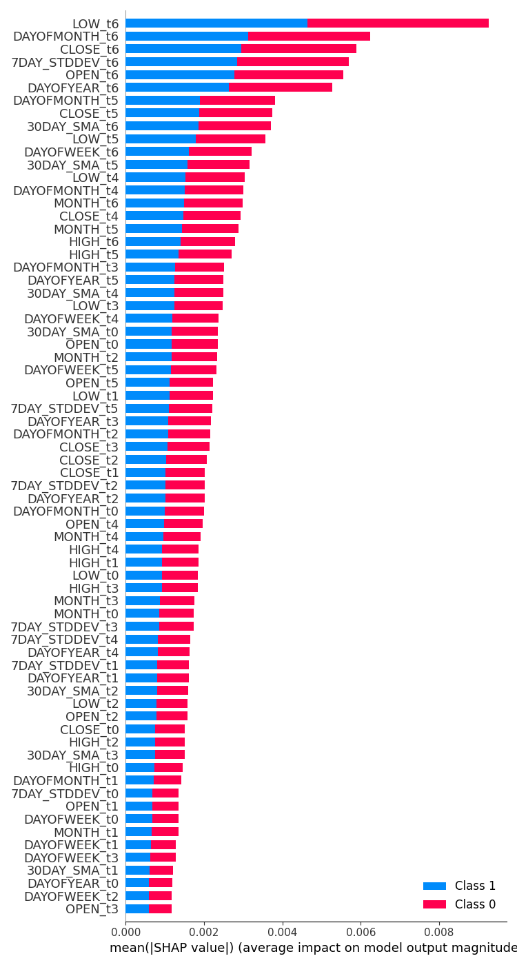 | feature_importance = gru_clf.check_feature_importance(X.columns) Outcome.  |
The LSTM classifier feature importance looks somehow similar to the one we obtained with the simple RNN model. The least important variables are from far time steps meanwhile the most important features are ones from closer timesteps.
This is like saying, that the variables that contribute the most to what happens to the current bar are the recent closed bar information.
The GRU classifier had a diverse opinion that doesn't seem to make much sense. This could be because its model had a lower accuracy.
It said the most impactful variable was the day of the week 7 days prior. Features such as Open, High, Low,, and Close from the time step value of 6 which is the very recent information, were placed in the middle indicating they had an average contribution to the final prediction outcome.
LSTM Versus GRU classifiers on the Strategy Tester
Shortly after training, both LSTM and GRU classifier models were saved to ONNX format.
LSTM | Python
lstm_clf.build_compile_and_train(best_params, verbose=1) # best_params = best parameters obtained after optimization

lstm_clf.save_onnx_model("lstm.EURUSD.D1.onnx")
GRU | Python
gru_clf.build_compile_and_train(best_params, verbose=1)

gru_clf.save_onnx_model("gru.EURUSD.D1.onnx") # best_params = best parameters obtained after optimization
After saving the ONNX model and its scaler files under the MQL5\Files directory, we can add the files to both Expert Advisors as resource files.
| LSTM | GRU |
|---|---|
#resource "\\Files\\lstm.EURUSD.D1.onnx" as uchar onnx_model[]; //lstm model in onnx format #resource "\\Files\\lstm.EURUSD.D1.standard_scaler_mean.bin" as double standardization_mean[]; #resource "\\Files\\lstm.EURUSD.D1.standard_scaler_scale.bin" as double standardization_std[]; #include <MALE5\Recurrent Neural Networks(RNNs)\LSTM.mqh> CLSTM lstm; #include <MALE5\preprocessing.mqh> StandardizationScaler *scaler; //For loading the scaling technique | #resource "\\Files\\gru.EURUSD.D1.onnx" as uchar onnx_model[]; //gru model in onnx format #resource "\\Files\\gru.EURUSD.D1.standard_scaler_mean.bin" as double standardization_mean[]; #resource "\\Files\\gru.EURUSD.D1.standard_scaler_scale.bin" as double standardization_std[]; #include <MALE5\Recurrent Neural Networks(RNNs)\GRU.mqh> CGRU gru; #include <MALE5\preprocessing.mqh> StandardizationScaler *scaler; //For loading the scaling technique |
The code for the rest of the Expert Advisors remains the same as we discussed.
Using default settings we have used since Part 24 of this article series, where we started with Timeseries forecasting.
Stop loss: 500, Take profit: 700, Slippage: 50.
Again, since the data was collected on a daily timeframe it might be a good idea to test it on a lower timeframe to avoid errors when "market closed errors" since we are looking for trading signals at the opening of a new bar. We can also set the Modelling type to open prices for faster testing.

LSTM Expert Advisor results


GRU Expert Advisor results


What can we learn from the Strategy Tester outcomes
Despite being the least accurate model with 44.98%, LSTM-based Expert Advisor was the most profitable with a net profit of 138 $, followed by the GRU-based Expert Advisor which was profitable 45.25% of the time, despite giving a total net profit of 120 $.
LSTM is a clear winner in this case profits-wise. Despite LSTM being technically smarter than other RNNs of its kind, there could be a lot of factors leading to this all recurrent models are good and can outperform others in certain situations, feel free to use any of the models discussed in this and the previous article.
The Differences Between LSTM and GRU Neural Network Models
Understanding these models in comparison helps when deciding what each model offers in contrast to the other. When one should be used, and when it shouldn't. Below are their tabulated differences.
| Aspect | LSTM | GRU |
|---|---|---|
Architecture Complexity | LSTMs have a more complex design with three gates (input, output, forget) and a cell state, providing detailed control over what information is kept or discarded at each time step. | GRUs have a simpler design with only two gates (reset and update). This simple architecture makes them easier to implement. |
Training Speed | Having additional gates and a cell state in LSTMs means there is more process to be done and parameters to optimize. They are slower during training. | Due to having fewer with fewer gates and simpler operations, they typically train faster than LSTMs. |
Performance | In complex problems where capturing long-term dependencies is crucial LSTMs tend to perform slightly better than their counterparts. | GRUs usually deliver comparable performance to LSTMs for many tasks. |
Handling of Long-Term Dependencies | LSTMs are explicitly designed to retain long-term dependencies in the data, thanks to the cell state and the gating mechanisms that control information flow over time. | While GRUs also handle long-term dependencies well, they may not be as effective as LSTMs in capturing very long-term dependencies due to their simpler structure. |
| Memory Usage | Due to their complex structure and additional parameters, LSTMs consume more memory, which can be a limitation in resource-constrained environments. | GRUs on the other hand are simpler, have fewer parameters, and uses less memory. Making them more suitable for applications with limited computational resources. |
Final Thoughts
Both LSTM (Long Short-Term Memory) and GRU (Gated Recurrent Unit) neural networks are powerful tools for traders seeking to leverage advanced time-series forecasting models. While LSTMs provide a more intricate architecture that excels at capturing long-term dependencies in market data, GRUs offer a simpler and more efficient alternative that can often match the performance of LSTMs with less computational costs.
These Timeseries deep learning models(LSTM and GRU), have been utilized in various domains outside forex trading such as weather forecasting, energy consumption modeling, anomaly detection, and speech recognition with great success as usually hyped however, In the forever-changing forex market I can not guarantee such promises.
This article aimed only to provide an understanding of these models in depth and how they can be deployed in MQL5 for trading. Feel free to explore and play with the models and datasets discussed in this article and share your results in the discussion section.
Best regards.
Track development of machine learning models and much more discussed in this article series on this GitHub repo.
Attachments Table
| File name | File type | Description & Usage |
|---|---|---|
| GRU EA.mq5 LSTM EA.mq5 | Expert Advisors | GRU based Expert Advisor. LSTM based Expert Advisor. |
| gru.EURUSD.D1.onnx lstm.EURUSD.D1.onnx | ONNX files | GRU model in ONNX format. LSTM model in ONNX format. |
| lstm.EURUSD.D1.standard_scaler_mean.bin lstm.EURUSD.D1.standard_scaler_scale.bin | Binary files | Binary files for the Standardization scaler used for the LSTM model. |
| gru.EURUSD.D1.standard_scaler_mean.bin gru.EURUSD.D1.standard_scaler_scale.bin | Binary files | Binary files for the Standardization scaler used for the GRU model. |
| preprocessing.mqh | An Include file | A library which consists of the Standardization Scaler. |
| lstm-gru-for-forex-trading-tutorial.ipynb | Python Script/Jupyter Notebook | Consists all the python code discussed in this article |
- Illustrated Guide to LSTM's and GRU's: A step by step explanation
- Designing neural network based decoders for surface codes
- An Adaptive Anti-Noise Neural Network for Bearing Fault Diagnosis Under Noise and Varying Load Conditions
Warning: All rights to these materials are reserved by MetaQuotes Ltd. Copying or reprinting of these materials in whole or in part is prohibited.
This article was written by a user of the site and reflects their personal views. MetaQuotes Ltd is not responsible for the accuracy of the information presented, nor for any consequences resulting from the use of the solutions, strategies or recommendations described.

- Free trading apps
- Over 8,000 signals for copying
- Economic news for exploring financial markets
You agree to website policy and terms of use