Data Science and Machine Learning (Part 24): Forex Time series Forecasting Using Regular AI Models

Contents

• What is time series forecasting?
• Why and where time series forecasting is used?
• A comparison between classical and modern against time series-based ML models
• Feature engineering for time series forecasting
• Training the LightGBM regressor model
• Augmented Dickey-Fuller test
• Why does stationarity matter?
• Predicting a stationary target variable
• Building the LightGBM classifier model
• Saving LightGBM Classifier Model to ONNX
• Wrapping it all Up Inside a Trading Robot
• Testing the model in the strategy tester
• Advantages of using classical and modern ML models for time series forecasting
• Conclusion

What is Time series Forecasting?

Time series forecasting is the process of using past data to predict future values in a sequence of data points. This sequence is typically ordered by time, hence the name time series.

Core Variables in Time series data 

While we can have as many feature variables as we want in our data, any data for time series analysis or forecasting must have these two variables.

1. Time
   
    This is an independent variable, representing the specific points in time when the data points were observed.
   
   
2. Target Variable
   
   This is the value you're trying to predict based on past observations and potentially other factors. (e.g., Daily closing stock price, hourly temperature, website traffic per minute).

The goal of time series forecasting is to leverage historical patterns and trends within the data to make informed predictions about future values.

This article assumes you have a basic understanding of ONNX, Time series forecasting, and Light Gradient Boosting Machine(LightGBM). Kindly read these articles if you haven't for clarity purposes. 

Why and Where Time Series Forecasting is Used?

Time series analysis and forecasting can be used  in the below scenarios:

• Forecasting future values 
• Understanding the past behavior(s)
• Planning for the future, which could be dependent on the past
• Evaluating current accomplishments

Classical and modern vs Time Series-Based Machine Learning Models

Unlike classic machine learning models such as Linear Regression, Support Vector Machine (SVM), Neural Networks (NN) and others, that we have discussed in prior articles — which aim to determine relationships among feature variables and make future predictions based on these learned relationships — time series models forecast future values based on previously observed values.

This difference in approach means that time series models are specifically designed to handle temporal dependencies and patterns inherent in sequential data. Time series forecasting models, such as ARIMA, SARIMA, Exponential Smoothing, RNN, LSTM, and GRU, leverage historical data to predict future points in the series, capturing trends, seasonality, and other temporal structures.

The flowchart below illustrates various machine learning models used for time series forecasting, 

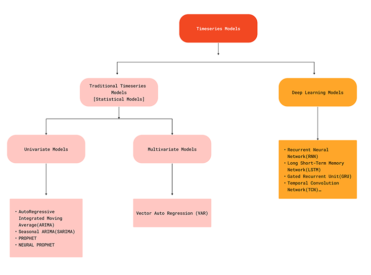
Since the Time series models are capable of capturing temporal dependencies in the data, they can offer a realistic solution when trying to make predictions on the forex market as we all know what happens currently in the market might be due to some factors that have just happened shortly or somewhere in the past. For example, news released on EURUSD 5 minutes ago might be one of the factors for a sharp price change at the current time. To understand this better let us look at the advantages of Time series forecasting in contrast to traditional forecasting using machine learning models.

Aspect	Time Series Forecasting	Traditional and Modern ML forecasting
Temporal Dependencies	Are capable of capturing temporal patterns since they consider the order of data points and dependencies over time.	Traditional ML models treat data points as independent,  ignoring temporal dependencies in the data in doing so.
Trend and Seasonality Handling	Time series models like ARIMA and some others have built-in components to handle trends and seasonality	Requires manual extraction and engineering of features to capture trends and seasonality.
Autocorrelation	Models like ARIMA and LSTMs can account for autocorrelation in the data.	They assume every feature is independent, so they may not account for autocorrelation unless explicitly modeled in features.
Model Complexity	Time series models are designed for sequential data, providing a more natural fit for such tasks.	Traditional models may require feature engineering to handle sequential data appropriately. This adds complexity to the process
Temporal Hierarchies	Can naturally extend to hierarchical time series forecasting (e.g., monthly, weekly).	Traditional models may struggle with forecasting at multiple temporal scales without additional engineering.
Predictive Performance	Often yields better predictive performance on time-dependent tasks due to consideration of order.	May underperform on time-dependent tasks.
Computational Efficiency	Time series models can incrementally update with new data efficiently.	Traditional models may need complete retraining, which is computationally more intensive with new data.
Interpretable Trends and Seasonality	Models like ARIMA provide interpretable components for trend and seasonality.	Requires additional steps to interpret trends and seasonality from engineered features.

Despite not being good at time series forecasting by default, classical and modern machine learning models like LightGBM, XGBoost, CatBoost, etc. can still be used for time series predictions when given the right information. The key to achieving this lies in feature engineering.

Feature Engineering for Time Series Forecasting

In time series forecasting, the aim is to build new features and prepare existing features in such a way they end up with important information/components for time series such as: Trend, Seasonality, Cyclic Patterns, Stationarity, Autocorrelation and Partial Autocorrelation, etc.

There are many aspects you can consider when making new features for a time series problem, below are some of those:

01: Lagged Features

In the data for classical machine learning, we often collect data like OPEN, HIGH, LOW, CLOSE, and some other data at the current bar. This contains the current information at every particular bar and offers no information on what happened before that specific bar.

By introducing lagged features to our data we ensure to capture temporal dependencies from prior bars which definitely has something to do with the current bar price.

MQL5

//--- getting Open, high, low and close prices
   
   ohlc_struct OHLC;
   
   OHLC.AddCopyRates(Symbol(), timeframe, start_bar, bars);
   time_vector.CopyRates(Symbol(), timeframe, COPY_RATES_TIME, start_bar, bars);
   
//--- Getting the lagged values of Open, High, low and close prices

   ohlc_struct  lag_1;
   lag_1.AddCopyRates(Symbol(), timeframe, start_bar+1, bars);
   
   ohlc_struct  lag_2;
   lag_2.AddCopyRates(Symbol(), timeframe, start_bar+2, bars);
   
   ohlc_struct  lag_3;
   lag_3.AddCopyRates(Symbol(), timeframe, start_bar+3, bars);

In the above example we are only getting three lags. Since we are collecting this data daily, We are getting the three prior days information for 1000 bars.

By Copying MqlRates in vectors starting at start_bar+1 we are getting one bar previous than copying rates starting at start_bar. This can be confusing sometimes kindly refer to https://www.mql5.com/en/docs/series

MQL5

input int bars = 1000;
input ENUM_TIMEFRAMES timeframe = PERIOD_D1;
input uint start_bar = 2; //StartBar|Must be >= 1

struct ohlc_struct 
{
   vector open;
   vector high;
   vector low;
   vector close;
   
   matrix MATRIX; //this stores all the vectors all-together
   
   void AddCopyRates(string symbol, ENUM_TIMEFRAMES tf, ulong start, ulong size)
    {
      open.CopyRates(symbol, tf, COPY_RATES_OPEN, start, size); 
      high.CopyRates(symbol, tf, COPY_RATES_HIGH, start, size); 
      low.CopyRates(symbol, tf, COPY_RATES_LOW, start, size); 
      close.CopyRates(symbol, tf, COPY_RATES_CLOSE, start, size); 
      
      this.MATRIX.Resize(open.Size(), 4); //we resize it to match one of the vector since all vectors are of the same size
      
      this.MATRIX.Col(open, 0);
      this.MATRIX.Col(high, 1);
      this.MATRIX.Col(low, 2);
      this.MATRIX.Col(close, 3);
    }
};

02: Rolling Statistics

Rolling statistics such as the mean, standard deviations, and other statistics of this kind help summarize recent trends and volatility within a window. This is where some indicators come into play such as the moving average for a certain period, the standard deviation for a given time, etc.

int ma_handle = iMA(Symbol(),timeframe,30,0,MODE_SMA,PRICE_WEIGHTED); //The Moving averaege for 30 days
int stddev = iStdDev(Symbol(), timeframe, 7,0,MODE_SMA,PRICE_WEIGHTED); //The standard deviation for 7 days
   
vector SMA_BUFF, STDDEV_BUFF;
SMA_BUFF.CopyIndicatorBuffer(ma_handle,0,start_bar, bars);
STDDEV_BUFF.CopyIndicatorBuffer(stddev, 0, start_bar, bars);

These rolling statistics provide a broader picture of how the market has been changing, potentially capturing long-term fluctuations that are not evident in the lagged features.

03: Date-Time Features

As said earlier time series data has the time variable however, having a Date-time variable only is not going to help much, we need to extract its features.

As we know the forex market exhibits some patterns or behaves a certain ways during specific times. For example: there is usually not much trading activity on Friday and the market is volatile when there is a news event on that particular day. Also in some months the trading activities can change for better or worse, the same applies for some years. For example: during the election year(s) for some countries like the US elections.

By introducing the Date-Time features we explicitly capture seasonal patterns, this would allow our model to adjust predictions based on the time of a year, a specific day or month, etc.

Let us collect Date-Time features in MQL5:

vector time_vector; //we want to add time vector 
time_vector.CopyRates(Symbol(), timeframe, COPY_RATES_TIME, start_bar, bars); //copy the time in seconds


ulong size = time_vector.Size(); 
vector DAY(size), DAYOFWEEK(size), DAYOFYEAR(size), MONTH(size);

MqlDateTime time_struct;
string time = "";
for (ulong i=0; i<size; i++)
  {
    time = (string)datetime(time_vector[i]); //converting the data from seconds to date then to string
    TimeToStruct((datetime)StringToTime(time), time_struct); //convering the string time to date then assigning them to a structure
    
    DAY[i] = time_struct.day;
    DAYOFWEEK[i] = time_struct.day_of_week;
    DAYOFYEAR[i] = time_struct.day_of_year;
    MONTH[i] = time_struct.mon;
  }

04: Differencing

Differencing the series at seasonal lags removes seasonal patterns from the data to achieve stationarity which is often a requirement for some models.

Let us try differencing at lag1 from the current prices.

MQL5

vector diff_lag_1_open = OHLC.open - lag_1.open;
vector diff_lag_1_high = OHLC.high - lag_1.high;
vector diff_lag_1_low = OHLC.low - lag_1.low;
vector diff_lag_1_close = OHLC.close - lag_1.close;

You can differentiate as many lags as you want, you are not restricted to lag 1 only.

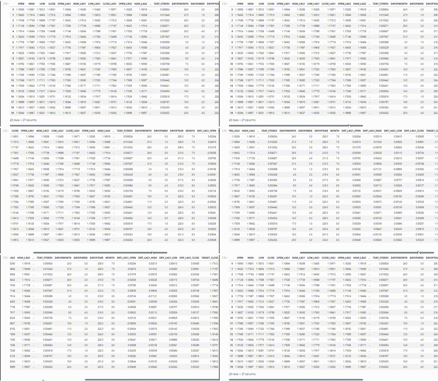
To this point we are having 26 independent variables/features that is enough for our independent variables. Since we are trying to solve a regression problem let us collect the close prices as our final target variable.

vector TARGET_CLOSE;
TARGET_CLOSE.CopyRates(Symbol(), timeframe, COPY_RATES_CLOSE, start_bar-1, bars); //one bar forward

Feel free to create more features for your problem by considering some other aspects we haven't considered below.

05: External Variables (Exogenous Features)

• Weather Data: try to see if it helps
• Economic Indicators: including GDP, unemployment rates, etc., for financial forecasting.

06: Fourier and Wavelet Transforms

Using Fourier or wavelet transforms to extract cyclical patterns and trends in the frequency domain.

07: Target Encoding

You can create features based on aggregate statistics (mean, median) of the target variable over different time-periods.

The final dataset has 27 columns:

Training the LightGBM Regressor Model

Now that we have all the data we need let us shift to the Python side of things.

We can start by splitting the data into training and testing samples.

Python

X = df.drop(columns=["TARGET_CLOSE"])
Y = df["TARGET_CLOSE"]

train_size = 0.7 #configure train size

train_size = round(train_size*df.shape[0])

x_train = X.iloc[:train_size,:]
x_test = X.iloc[train_size:, :]

y_train = Y.iloc[:train_size]
y_test = Y.iloc[train_size:]

print(f"x_train_size{x_train.shape}\nx_test_size{x_test.shape}\n\ny_train{y_train.shape}\ny_test{y_test.shape}")

Outcomes

x_train_size(700, 26)
x_test_size(300, 26)

y_train(700,)
y_test(300,)

Let us fit the model to the training data.

model = lgb.LGBMRegressor(**params)
model.fit(x_train, y_train)

Let us test the trained model then plot the predictions and the r2_score.

Python

from sklearn.metrics import r2_score

test_pred = model.predict(x_test)

accuracy = r2_score(y_test, test_pred)

#showing actual test values and predictions

plt.figure(figsize=(8, 6))  
plt.plot(y_test, label='Actual Values')
plt.plot(test_pred, label='Predicted Values')
plt.xlabel('Index')
plt.ylabel('Values')
plt.title('Actual vs. Predicted Values')
plt.legend(loc="lower center")

# Add R-squared (accuracy) score in a corner
plt.text(0.05, 0.95, f"LightGBM (Accuracy): {accuracy:.4f}", ha='left', va='top', transform=plt.gca().transAxes, fontsize=10, bbox=dict(boxstyle='round', facecolor='white', alpha=0.7))

plt.grid(True)

plt.savefig("LighGBM Test plot")
plt.show()

Outcome

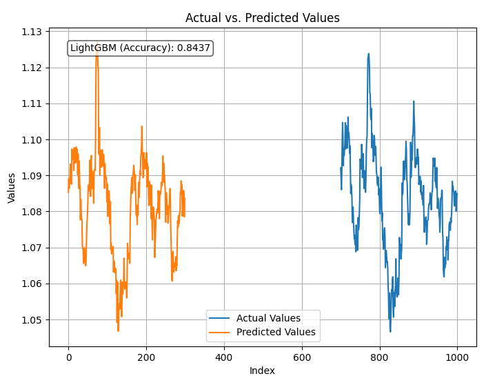
The model is 84% accurate predicting the close prices using all the data it was given. While this seems to be a good accuracy we need to examine our variables for further analysis and model improvement.

Using the built-in LightGBM feature importance plotting technique, below is the plot for feature importance.

Python

# Plot feature importance using Gain
lgb.plot_importance(model, importance_type="gain", figsize=(8,6), title="LightGBM Feature Importance (Gain)")

plt.tight_layout()

plt.savefig("LighGBM feature importance(Gain)")
plt.show()

Outcome:

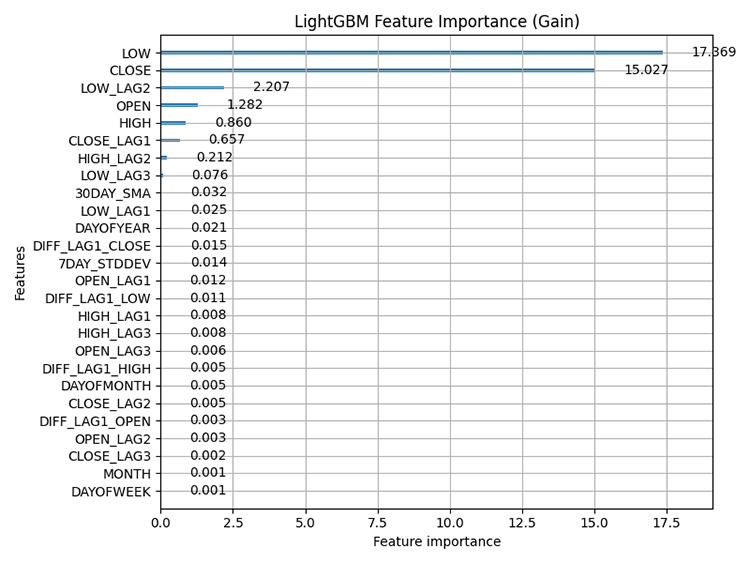
Feature importance: refers to techniques that assess the relative contribution of each feature(variable) in a dataset to the predictions made by the model. It helps us understand which features have the most significant influence on the model's predictions.

It is important to know that tree-based methods such LightGBM and XGBoost calculate feature importance differently than non-tree-based models, they consider how often a feature is used for splitting decisions in the trees and the impact of those splits on the final prediction.

Alternatively, you can use SHAP to check for feature importance.

Python:

explainer = shap.TreeExplainer(model)
shap_values = explainer(x_train)  

shap.summary_plot(shap_values, x_train, max_display=len(x_train.columns), show=False)  # Show all features

# Adjust layout and set figure size
plt.subplots_adjust(left=0.12, bottom=0.1, right=0.9, top=0.9)  
plt.gcf().set_size_inches(6, 8) 
plt.tight_layout()

plt.savefig("SHAP_Feature_Importance_Summary_Plot.png")
plt.show()

Outcome:

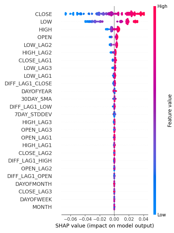
From feature importance plots, it is clear that the variables for capturing seasonal patterns such as DAYOFWEEK, MONTH, DAYOFMONTH, and DAYOFYEAR are some of the variables with the least contribution to the model's predictions.

Strangely enough, all these are stationary according to the Augmented Dickey Fuller test.

  

Augmented Dickey-Fuller (ADF) Test

This is a statistical test used to determine whether a time series dataset is stationary or not. Stationarity is a crucial property for many time series forecasting and analysis methods.

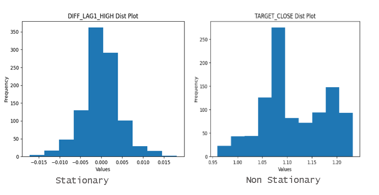
A stationary variable or a stationary dataset refers to a series where the statistical properties (mean, variance, autocorrelation) remain constant over time. For-example in the stock market. The mean of the OHLC values may increase or decrease drastically over time making these values non-stationary for the most part meanwhile, their returns such as the mean or variance of the difference between High and Low are stationary over time.

I ran this test on the entire dataset we have.

from statsmodels.tsa.stattools import adfuller

def adf_test(series, signif=0.05):
  """
  Performs the ADF test on a pandas Series and interprets the results.

  Args:
      series: The pandas Series containing the time series data.
      signif: Significance level for the test (default: 0.05).

  Returns:
      A dictionary containing the test statistic, p-value, used lags,
      critical values, and interpretation of stationarity.
  """
  dftest = adfuller(series, autolag='AIC')
  adf_stat = dftest[0]  # Access test statistic
  pvalue = dftest[1]  # Access p-value
  usedlag = dftest[2]  # Access used lags
  critical_values = dftest[4]  # Access critical values

  interpretation = 'Stationary' if pvalue < signif else 'Non-Stationary'
  result = {'Statistic': adf_stat, 'p-value': pvalue, 'Used Lags': usedlag,
            'Critical Values': critical_values, 'Interpretation': interpretation}
  return result

for col in df.columns:
  adf_results = adf_test(df[col], signif=0.05)
  print(f"ADF Results for column {col}:\n {adf_results}")

Out of 27 Variables, only 9 variables were detected stationary. These variables are: 

1. 7DAY_STDDEV
2. DAYOFMONTH
3. DAYOFWEEK
4. DAYOFYEAR
5. MONTH
6. DIFF_LAG1_OPEN
7. DIFF_LAG1_HIGH
8. DIFF_LAG1_LOW
9. DIFF_LAG1_CLOSE

To easily find out if the variables are stationary or not you can simply look at the distribution plot. A data well distributed around the mean is most likely a stationary data.

Why does Stationarity Matter?

Many statistical methods utilized in time series analysis and forecasting assume stationarity. If a time series is non-stationary these methods can produce misleading or inaccurate results. 

Imagine trying to forecast future stock prices if the prices are constantly trending upwards. The Time series model wouldn't be able to capture the underlying trend.

Classical or even the so called modern machine learning models such as the LightGBM we used have the ability to handle non-linear relationships between the features making them less affected by the stationarity present in the data. The feature importance for this model has clearly demonstrated that the most important features for our model are non-stationary OHLC variables.

However, this doesn't mean variables such as day of the week have no impact on the model. Feature importance is just one part of the big story, domain knowledge is still required In my opinion.

There is no need to drop this variable because it is ranked lower as I am confident it affects the EURUSD. 

Predicting a Stationary Target Variable

Having a stationary target variable improves the performance of many machine learning models when it comes to time series forecasting since stationary data has a constant (mean, variance, autocorrelation) over time. As you know predicting where the market will move in the next candle is difficult but predicting the amount of pips or points for the next move isn't very difficult.

If we can predict the amount of points the next bar will generate we can use this to set trading targets (Stop loss and Take profit).

To achieve this we need to find first order differencing, by subtracting the previous close price from the next close price.

Python

Y = df["TARGET_CLOSE"] - df["CLOSE"] #first order differencing 

By differencing the next close prices to the prior ones we end up with stationary variable.

adf_results = adf_test(Y,signif=0.05)

print(f"ADF Results:\n {adf_results}")

Results:

ADF Results: {'Statistic': -23.37891429248752, 'p-value': 0.0, 'Used Lags': 1, 'Critical Values': {'1%': -3.4369193380671, '5%': -2.864440383452517, '10%': -2.56831430323573}, 'Interpretation': 'Stationary'}

After fitting the regressor model to the new stationary target variable and evaluating its performance on the test dataset, below was the outcome.

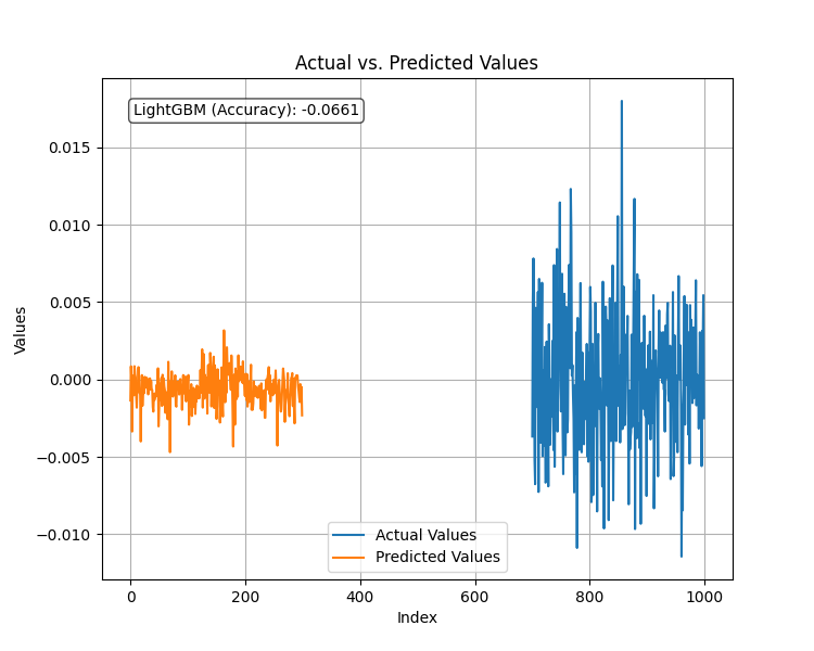
The model had a terrible performance when the target variable was a stationary one. As always in machine learning there could be many factors leading to this but for now we are going to conclude that LightGBM doesn't perform well for stationary target variables. We are going to stick with the regression model produced for predicting the target close values.

Having this regression model which predicts continuous close price values isn't as useful as having a model that predicts the trading signals such as buy or sell, to achieve this we need to make another model for predicting the trading signals.

Building the LightGBM Classifier Model

To make a classifier model, we need to prepare the target variable as a binary target variable where 1 represents a buy signal while 0 represents a sell signal.

Python

Y = []
target_open = df["TARGET_OPEN"]
target_close = df["TARGET_CLOSE"]

for i in range(len(target_open)):
    if target_close[i] > target_open[i]: # if the candle closed above where it opened thats a buy signal
        Y.append(1)
    else: #otherwise it is a sell signal
        Y.append(0)

# split Y into irrespective training and testing samples 

y_train = Y[:train_size]
y_test = Y[train_size:]

I trained the LightGBM model inside a Pipeline with the StandardScaler technique.

Python

from sklearn.pipeline import Pipeline
from sklearn.preprocessing import StandardScaler

params = {
    'boosting_type': 'gbdt',  # Gradient Boosting Decision Tree
    'objective': 'binary',  # For binary classification (use 'regression' for regression tasks)
    'metric': ['auc','binary_logloss'],  # Evaluation metric
    'num_leaves': 25,  # Number of leaves in one tree
    'n_estimators' : 100, # number of trees
    'max_depth': 5,
    'learning_rate': 0.05,  # Learning rate
    'feature_fraction': 0.9  # Fraction of features to be used for each boosting round
}

pipe = Pipeline([
    ("scaler", StandardScaler()),
    ("lgbm", lgb.LGBMClassifier(**params))
])

# Fit the pipeline to the training data
pipe.fit(x_train, y_train)

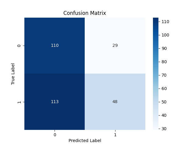
The testing results were not that surprising 53% overall accuracy.

Classification report:

Classification Report
               precision    recall  f1-score   support

           0       0.49      0.79      0.61       139
           1       0.62      0.30      0.40       161

    accuracy                           0.53       300
   macro avg       0.56      0.54      0.51       300
weighted avg       0.56      0.53      0.50       300

Confusion Matrix

Saving LightGBM Classifier Model to ONNX

As we did previously,  saving the LightGBM model to ONNX format is straightforward and requires only a few lines of code.

import onnxmltools
from onnxmltools.convert import convert_lightgbm
import onnxmltools.convert.common.data_types
from skl2onnx.common.data_types import FloatTensorType
from skl2onnx import convert_sklearn, update_registered_converter

from skl2onnx.common.shape_calculator import (
    calculate_linear_classifier_output_shapes,
)  # noqa

from onnxmltools.convert.lightgbm.operator_converters.LightGbm import (
    convert_lightgbm,
)  # noqa

# registering onnx converter

update_registered_converter(
    lgb.LGBMClassifier,
    "GBMClassifier",
    calculate_linear_classifier_output_shapes,
    convert_lightgbm,
    options={"nocl": [False], "zipmap": [True, False, "columns"]},
)

# Final LightGBM conversion to ONNX

model_onnx = convert_sklearn(
    pipe,
    "pipeline_lightgbm",
    [("input", FloatTensorType([None, x_train.shape[1]]))],
    target_opset={"": 12, "ai.onnx.ml": 2},
)

# And save.
with open("lightgbm.Timeseries Forecasting.D1.onnx", "wb") as f:
    f.write(model_onnx.SerializeToString())

Wrapping it all Up Inside a Trading Robot

Now that we have a machine learning model saved to ONNX, we can directly attach it inside an Expert Advisor and use the LightGBM classifier for time series predictions in MetaTrader 5.

MQL5

#resource "\\Files\\lightgbm.Timeseries Forecasting.D1.onnx" as uchar lightgbm_onnx[] //load the saved onnx file 
#include <MALE5\LightGBM\LightGBM.mqh>
CLightGBM lgb;

Using the LightGBM class built in the prior article, I was able to initialize the model and use it to make predictions.

int OnInit()
  {
//---
   
   if (!lgb.Init(lightgbm_onnx)) //Initialize the LightGBM model
     return INIT_FAILED;
   
//---
   return(INIT_SUCCEEDED);
  }
//+------------------------------------------------------------------+
//| Expert tick function                                             |
//+------------------------------------------------------------------+
void OnTick()
  {
//---
    
   if (NewBar()) //Trade at the opening of a new candle
    {
     vector input_vector = input_data(); 
     long signal = lgb.predict_bin(input_vector);
     
   //---
     
      MqlTick ticks;
      SymbolInfoTick(Symbol(), ticks);
      
      if (signal==1) //if the signal is bullish
       {
          if (!PosExists(POSITION_TYPE_BUY)) //There are no buy positions
           {
             if (!m_trade.Buy(lotsize, Symbol(), ticks.ask, ticks.bid-stoploss*Point(), ticks.ask+takeprofit*Point())) //Open a buy trade
               printf("Failed to open a buy position err=%d",GetLastError());
           }
       }
      else if (signal==0) //Bearish signal
        {
          if (!PosExists(POSITION_TYPE_SELL)) //There are no Sell positions
            if (!m_trade.Sell(lotsize, Symbol(), ticks.bid, ticks.ask+stoploss*Point(), ticks.bid-takeprofit*Point())) //open a sell trade
               printf("Failed to open a sell position err=%d",GetLastError());
        }
      else //There was an error
        return;
    }
  }

The input_data() function is responsible for collective data in a similar fashion to the way data was collected and stored in a CSV file in the script Feature engineering Timeseries forecasting.mq5. 

Testing the Model in the Strategy Tester.

Finally, we can test the model in the trading environment. Since the data was collected on a daily timeframe it might be a good idea to test it on a lower timeframe to avoid errors when "market closed errors" since we are looking for trading signal at the opening of a new bar. We can also set the Modelling type to open prices for faster testing.

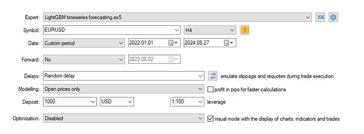
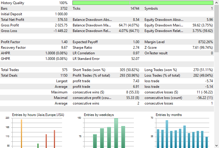
The EA made the correct predictions approximately 51% of the time, given the Stop loss and Take profit of 500 and 700 Points respectively.

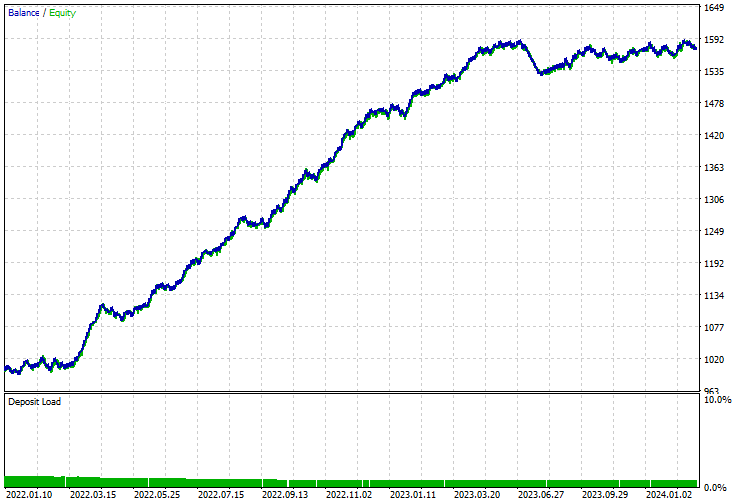
The balance/equity curve was impressive too.

Advantages of Using Classical and Modern ML models for Time series forecasting

Using non-time series machine learning models for time series forecasting has several advantages. Below are some key benefits:

1. Flexibility in Feature Engineering

Classical machine learning models allow extensive feature engineering, which can be leveraged to include various external variables and derived features. You can use your human intellect to manually analyze and incorporate all the data you deem useful including complex features such as lags and rolling statistics as we did in this post.

2. Handling Non-Stationarity

Instead of making the series stationary through differencing, you can include trend and seasonality directly as features and the model will learn the patterns without any issues.

3. No Assumptions About Data Distribution

Many classical time series models (like ARIMA) assume the data follows a specific statistical distribution. Classical and modern ML models on the other hand, are more flexible regarding data distribution.

Models like decision trees, random forests, and gradient boosting (including LightGBM) do not assume any specific distribution of the data.

4. Scalability

Classical ML models can handle large datasets more efficiently and are often easier to scale.

5. Complex Interactions

Classical ML models can capture complex, non-linear relationships between features and the target variable.

6. Robustness to Missing Data

Machine learning models often have better mechanisms for handling missing data compared to traditional time series models.

7. Ensemble Methods

You can easily use ensemble methods such as bagging, boosting, and stacking to enhance model performance by combining multiple models to improve predictive performance and robustness.

8. Ease of Use and Integration

Classical ML models are often more user-friendly and come with extensive libraries and tools for implementation, visualization, and evaluation.

Libraries like Scikit-learn, LightGBM, and XGBoost provide comprehensive tools for building, tuning, and evaluating these models.

The Bottom Line

Classical and modern machine learning models can both be used for time series analysis and forecasting without a problem and they can outperform time series models with the right information, tuning, and processes as discussed in this article. I decided to use LightGBM as an example however, any classical or modern machine learning model such as SVM, Linear Regression, Naïve Bayes, XGBoost, etc. can be applied.

Peace out.

Track development of machine learning models and much more discussed in this article series on this GitHub repo.

Attachments Table

File name	File type	Description & Usage
LightGBM timeseries forecasting.mq5	Expert Advisor	Trading robot for loading the ONNX model and testing the final trading strategy in MetaTrader 5.
lightgbm.Timeseries Forecasting.D1.onnx	ONNX	LightGBM model in ONNX format.
LightGBM.mqh	An Include (library)	Consists of the code for loading the ONNX model format and deploying it in native MQL5 language.
Feature engineering Timeseries forecasting.mq5	A Script	This is a script where all the data is collected and engineered for time series analysis and forecasting.
forex-timeseries-forecasting-lightgbm.ipynb	Python Script(Jupyter Notebook)	All the python code discussed in this article can be found inside this notebook.

Sources & References:

• Time Series Talk: Stationarity (https://youtu.be/oY-j2Wof51c)
• Kishan Manani - Feature Engineering for Time Series Forecasting | PyData London 2022 (https://www.youtube.com/watch?v=9QtL7m3YS9I)
• Stock Market Prediction via Deep Learning Techniques: A Survey (https://arxiv.org/abs/2212.12717)
• Challenges in Time Series Forecasting (https://www.youtube.com/watch?v=rcdDl8qf0ZA)
• Stationarity and differencing (https://otexts.com/fpp2/stationarity.html)
• How to perform Target/Mean Encoding for Categorical Attributes | Python (https://www.youtube.com/watch?v=nd7vc4MZQz4)