
Data Science and ML (Part 29): Essential Tips for Selecting the Best Forex Data for AI Training Purposes

Contents
- Introduction
- What is Feature Selection
- Why feature selection is necessary to AI models?
- Filter methods
Correlation Matrix
Statistical Tests
— Chi-squared test
— ANOVA test - Wrapper methods
Recursive feature elimination (RFE)
Sequential features selection (SFS) - Embedded methods
Lasso regression
Decision tree-based methods - Dimensionality reduction techniques
- Conclusion
Introduction
With all the trading data and information such as indicators (there are more than 36 built-in indicators in MetaTrader 5), symbol pairs (there are more than 100 symbols) that can also be used as data for correlation strategies, there are also news which are valuable data for traders, etc. The point I'm trying to raise is that there is abundant information for traders to use in manual trading or when trying to build Artificial Intelligence models to help us make smart trading decisions in our trading robots.
Out of all the information we have at hand, there has to be some bad information (that is just common sense). Not all indicators, data, strategy, etc. are useful for a particular trading symbol, strategy, or situation. How do we determine the right information for trading and machine learning models for maximum efficiency and profitability? This is where feature selection comes into play.
What is Feature Selection
Feature selection is a process of identifying and selecting a subset of relevant features from the original dataset to be used in model construction. This is a process of determining the most useful information to feed a machine learning model and dropping the garbage(less important features/information).
Feature selection is one of the critical steps in building an effective machine learning model, below are the reasons why.
Why Feature Selection is Necessary to AI Models?
- Reduces dimensionality
By eliminating irrelevant or redundant features, feature selection simplifies the model and reduces computational costs. - Enhances performance
Focusing on the most informative features can improve the accuracy and predictive power of the model. - Improves interpretability
Models with fewer features are often easier to understand and explain. - Handles noise by removing noisy or irrelevant data
By removing less important features, feature selection can help prevent overfitting which is often caused by having too much irrelevant data.
Now that we know how important feature selection is, let us explore different techniques that are often used by data scientists and machine learning experts to find the best features for their AI models.
Using the same dataset we used in this article (must-read), The dataset has 28 variables.

Out of 28 variables, we want to find the most relevant variables to the "TARGET_OPEN" (which holds the next candle's opening price values) and "TARGET_CLOSE" (which holds the next candle's closing price values) columns and leave behind the less irrelevant data.
Feature selection techniques and methods can be categorized into three main types; filter methods, wrapper methods, and embedded methods. Let us dissect one method one after the other to see what they are all about.
Filter Methods
Filter methods evaluate features independently of the machine learning model or algorithm. These methods include the use of the correlation matrix and performing statistical tests.
Correlation Matrix
A correlation matrix is a table that shows the correlation coefficients between different variables.
A correlation coefficient is a statistical measure that indicates the strength and direction of the relationship between two variables. It ranges from -1 to 1.
A value of 1 indicates a perfect positive correlation (as one variable increases, the other increases proportionally).
A value of 0 Indicates there is no correlation (no relationship between the two variables).-1
A value of -1 indicates a perfect negative correlation (as one variable increases, the other decreases proportionally).
Let us start by computing the correlation matrix using Python.
Computing the Correlation Matrix
# Compute the correlation matrix
corr_matrix = df.corr()

# We generate a mask for the upper triangle
mask = np.triu(np.ones_like(corr_matrix, dtype=bool))
cmap = sns.diverging_palette(220, 10, as_cmap=True) # Custom colormap


plt.figure(figsize=(28, 28)) # 28 columns to fit better

# Draw the heatmap with the mask and correct aspect ratio
sns.heatmap(corr_matrix, mask=mask, cmap=cmap, vmax=1.0, center=0, annot=True,
            square=True, linewidths=1, cbar_kws={"shrink": .75})

plt.title('Correlation Matrix')
plt.savefig("correlation matrix.png")
plt.show()
Outputs
The matrix is too huge to show, below are some of the very useful parts.

Identify and Eliminate Highly Correlated Features
High multicollinearity occurs when two or more features are highly correlated with each other, this can cause issues in many machine learning algorithms, particularly linear models, this situation leads to unstable estimates of the coefficients.
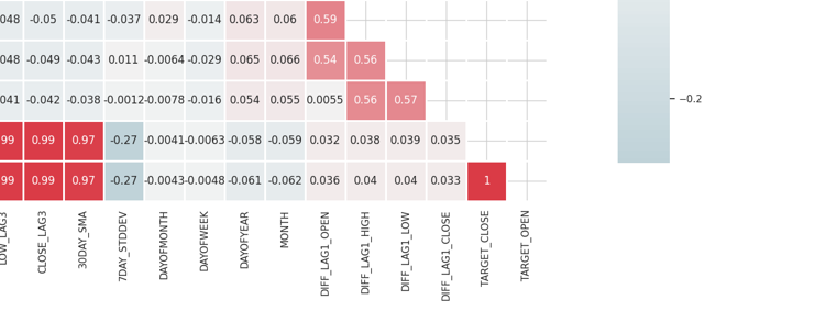
Correlation between Independent Variables Themselves
By combining or removing highly correlated features, you can simplify your model without losing much information. For example; In the correlation matrix image above, Open, High, and Low are 100% correlated. They are correlated 99.something % (these final values are rounded). We can decide to remove these variables and remain with only one variable, or use techniques to reduce the dimension of the data we are about to discuss.
Correlation between Independent variables (features) and the Target variable
Features that have a strong correlation with the target variable are generally more informative and can improve the predictive performance of the model.
The confusion matrix is not directly applicable to categorical features in our dataset such as "DAYOFWEEK", "DAYOFYEAR", and "MONTH" since correlation coefficients measure the linear relationships between numerical variables.
Statistical Tests
We can run statistical tests to select features with significant relationships to the target variable.
Chi-squared Test
The Chi-squared test measures how expected counts compare to the observed counts in a contingency table. It helps determine whether there is a significant association between two categorical variables.
A contingency table is a type of table in a matrix format that displays the frequency distribution of the variables, It can be used to examine the relationship between two categorical variables. Within the Chi-squared test, a contingency table is used to compare the observed frequencies of categorical variables against the expected frequencies.
The Chi-squared test is applicable to categorical variables only.
In our dataset, we have a couple of categorical variables (DAYOFMONTH, DAYOFWEEK, DAYOFYEAR, and MONTH). We also have to create a target variable to measure the relationships between it and the features.
Python codefrom sklearn.feature_selection import chi2 from sklearn.feature_selection import SelectKBest target = [] # Loop through each row in the DataFrame to create the target variable for i in range(len(df)): if df.loc[i, 'TARGET_CLOSE'] > df.loc[i, 'TARGET_OPEN']: target.append(1) else: target.append(0) X = pd.DataFrame({ 'DAYOFMONTH': df['DAYOFMONTH'], 'DAYOFWEEK': df['DAYOFWEEK'], 'DAYOFYEAR': df['DAYOFYEAR'], 'MONTH': df['MONTH'] }) chi2_selector = SelectKBest(chi2, k='all') chi2_selector.fit(X, target) chi2_scores = chi2_selector.scores_ # Output scores for each feature feature_scores = pd.DataFrame({'Feature': X.columns, 'Chi2 Score': chi2_scores}) print(feature_scores)
Outputs
      Feature  Chi2 Score
0  DAYOFMONTH    0.622628
1   DAYOFWEEK    0.047481
2   DAYOFYEAR   14.618057
3       MONTH    0.489713
From the outputs above, we see that DAYOFYEAR has the highest Chi2 score which indicates that it is the most impactful variable on the target variable compared to the others. This makes sense, as the data was collected from a daily timeframe, and each day uniquely corresponds to a day of the year. The strong presence of the DAYOFYEAR variable in the dataset likely increases its frequency and significance, making it a key feature in predicting the target variable.
ANOVA (Analysis of Variance) Test
ANOVA is a statistical method used to compare the means for three or more groups to see if at least one of the group means is statistically different from the others. It helps determine the strength of the relationship between continuous features and the categorical target variable.
It works by not only analyzing the variance within each group and between the groups but also, It measures the variability of observation within each group and the variability between the means of different groups.
This test calculates the F-statistic, which is the ratio of the between-group variance to the within-group variance. A higher F-statistic indicates that the groups have different means.
Let us use "f_classif" from Scikit-learn to perform an ANOVA test for feature selection.
Python code
from sklearn.feature_selection import f_classif

# We start by dropping the categorical variables in the dataset

X = df.drop(columns=[
    "DAYOFMONTH",
    "DAYOFWEEK",
    "DAYOFYEAR",
    "MONTH",
    "TARGET_CLOSE",
    "TARGET_OPEN"
])


# Perform ANOVA test

selector = SelectKBest(score_func=f_classif, k='all')
selector.fit(X, target)

# Get the F-scores and p-values
anova_scores = selector.scores_
anova_pvalues = selector.pvalues_

# Create a DataFrame to display results
anova_results = pd.DataFrame({'Feature': X.columns, 'F-Score': anova_scores, 'p-Value': anova_pvalues})
print(anova_results)
Outputs
            Feature   F-Score   p-Value
0              OPEN  3.483736  0.062268
1              HIGH  3.627995  0.057103
2               LOW  3.400320  0.065480
3             CLOSE  3.666813  0.055792
4         OPEN_LAG1  3.160177  0.075759
5         HIGH_LAG1  3.363306  0.066962
6          LOW_LAG1  3.309483  0.069181
7        CLOSE_LAG1  3.529789  0.060567
8         OPEN_LAG2  3.015757  0.082767
9         HIGH_LAG2  3.034694  0.081810
10         LOW_LAG2  3.259887  0.071295
11       CLOSE_LAG2  3.206956  0.073629
12        OPEN_LAG3  3.236211  0.072329
13        HIGH_LAG3  3.022234  0.082439
14         LOW_LAG3  3.020219  0.082541
15       CLOSE_LAG3  3.075698  0.079777
16        30DAY_SMA  2.665990  0.102829
17      7DAY_STDDEV  0.639071  0.424238
18   DIFF_LAG1_OPEN  1.237127  0.266293
19   DIFF_LAG1_HIGH  0.991862  0.319529
20    DIFF_LAG1_LOW  0.131002  0.717472
21  DIFF_LAG1_CLOSE  0.198001  0.656435
Higher F-scores indicate that the feature has a strong relationship with the target variable.
P-values less than the significant level (e.g. 0.05) are considered statistically significant.
We can also select the features with the highest F-scores or the lowest P-values which are the most important features and leave other features behind. Let us select the 10 top features.
Python code
selector = SelectKBest(score_func=f_classif, k=10)
X_selected = selector.fit_transform(X, target)


# print the selected feature names

selected_features = X.columns[selector.get_support()]
print("Selected Features:", selected_features)
Outputs
Selected Features: Index(['OPEN', 'HIGH', 'LOW', 'CLOSE', 'HIGH_LAG1', 'LOW_LAG1', 'CLOSE_LAG1',
       'LOW_LAG2', 'CLOSE_LAG2', 'OPEN_LAG3'],
      dtype='object')
Wrapper Methods
These methods involve evaluating the performance of a model using different subsets or features. Under wrapper methods, we are going to discuss Recursive Feature Elimination (RFE) and Sequential Feature Selection(SFS).
Recursive Feature Elimination (RFE)
This is a feature selection technique that aims to select the most relevant features by recursively considering smaller and smaller sets of features. It works by fitting a model and removing the least important features until the desired number of features is reached.
How RFE Works
We start by training any machine learning model. In this example; Let us use the Logistic Regression.
Python code
from sklearn.feature_selection import RFE
from sklearn.linear_model import LogisticRegression

# Prepare the target variable, again

y = []

# Loop through each row in the DataFrame to create the target variable
for i in range(len(df)):
    if df.loc[i, 'TARGET_CLOSE'] > df.loc[i, 'TARGET_OPEN']:
        y.append(1)
    else:
        y.append(0)

# Drop future variables from the feature set
X = df.drop(columns=["TARGET_CLOSE", "TARGET_OPEN"])

# Initialize the model
model = LogisticRegression(max_iter=10000)
We then initialize the RFE with the model and the number of most impactful features we want to select from the data.
# Initialize RFE with the model and number of features to select
rfe = RFE(estimator=model, n_features_to_select=10)

# Fit RFE
rfe.fit(X, y)
selected_features_mask = rfe.support_
Finally, we determine the least important features and eliminate them.
Python code
# Getting the names of the selected features
feature_names = X.columns
selected_feature_names = feature_names[selected_features_mask]


selected_features = pd.DataFrame({
    "Name": feature_names,
    "Mask": selected_features_mask
})

selected_features.head(-1)
Outputs
        Name    Mask
0       OPEN    True
1       HIGH    True
2       LOW     True
3       CLOSE   True
4       OPEN_LAG1       False
5       HIGH_LAG1       True
6       LOW_LAG1        True
7       CLOSE_LAG1      True
8       OPEN_LAG2       False
9       HIGH_LAG2       False
10      LOW_LAG2        True
11      CLOSE_LAG2      True
12      OPEN_LAG3       True
13      HIGH_LAG3       False
14      LOW_LAG3        False
15      CLOSE_LAG3      False
16      30DAY_SMA       False
17      7DAY_STDDEV     False
18      DAYOFMONTH      False
19      DAYOFWEEK       False
20      DAYOFYEAR       False
21      MONTH   False
22      DIFF_LAG1_OPEN  False
23      DIFF_LAG1_HIGH  False
24      DIFF_LAG1_LOW   False
All the features assigned the True value are the most important values. To obtain them, we can slice them from the original X matrix.
# Filter the dataset to keep only the selected features

X_selected = X.loc[:, selected_features_mask]

#for better readability, we convert this into pandas dataframe

X_selected_df = pd.DataFrame(X_selected, columns=selected_feature_names)

print("Selected Features")
X_selected_df.head()
Outputs

- RFE can be used with any model that can rank features by importance.
- By eliminating irrelevant features, RFE can improve the performance of the model.
- By Removing unnecessary features, it can help reduce overfitting
- It can be computationally expensive when given large datasets and complex models like neural networks, since it requires retraining the model multiple times.
- RFE is a greedy algorithm and may not always find the optimal subset of features.
Sequential Feature Selection(SFS)
This is a wrapper method for feature selection that incrementally builds a feature set by adding or removing features based on their performance contribution to a model. There are two main types of Sequential feature selection; Forward and backward elimination.
In forward selection, features are added one by one starting from an empty set until the desired number of features is reached, or adding more features does not improve the model performance.
In backward selection, this works opposite to the forward selection. We start with all features and remove them one by one, each time removing the least significant feature until the desired number of features is left.
Forward selection
from sklearn.feature_selection import SequentialFeatureSelector

# Create a logistic regression model
model = LogisticRegression(max_iter=10000)

# Create a SequentialFeatureSelector object
sfs = SequentialFeatureSelector(model, n_features_to_select=10, direction='forward')

# Fit the SFS object to the training data
sfs.fit(X, target)

# Get the selected feature indices
selected_features = sfs.get_support(indices=True)
selected_features_names = X.columns[selected_features] # get the feature names

# Print the selected features
print("Selected feature indices:", selected_features)
print("Selected feature names:", selected_feature_names)
Outputs
Selected feature indices: [ 1  7  8 12 17 19 22 23 24 25]
Selected feature names: Index(['OPEN', 'HIGH', 'LOW', 'CLOSE', 'HIGH_LAG1', 'LOW_LAG1', 'CLOSE_LAG1',
       'LOW_LAG2', 'CLOSE_LAG2', 'OPEN_LAG3'],
      dtype='object')
Backward selection
# Create a logistic regression model
model = LogisticRegression(max_iter=10000)

# Create a SequentialFeatureSelector object
sfs = SequentialFeatureSelector(model, n_features_to_select=10, direction='backward')

# Fit the SFS object to the training data
sfs.fit(X, target)

# Get the selected feature indices
selected_features = sfs.get_support(indices=True)
selected_features_names = X.columns[selected_features] # get the feature names

# Print the selected features
print("Selected feature indices:", selected_features)
print("Selected feature names:", selected_feature_names)
Outputs
Selected feature indices: [ 2  3  7 10 11 12 13 14 15 16]
Selected feature names: Index(['OPEN', 'HIGH', 'LOW', 'CLOSE', 'HIGH_LAG1', 'LOW_LAG1', 'CLOSE_LAG1',
       'LOW_LAG2', 'CLOSE_LAG2', 'OPEN_LAG3'],
      dtype='object')
Despite taking different approaches, both backward and forward methods converged to the same solution. Producing the same number of features.
- Easy to understand and implement.
- It can be used with any machine learning algorithm.
- Often leads to better model performance by selecting the most relevant features.
- This method is slow with large datasets or many features.
- May not find the optimal features set, as it makes decisions based on local improvements.
Embedded Methods
These methods involve performing feature selection during the model training process. Embedded feature selection workflow involves.
- Training a machine learning model
- Deriving feature importance
- Selecting the top ranking predictor variables
Lasso Regression
Linear regression models predict the outcome based on a linear combination of the feature space. The coefficients are determined by minimizing the squared difference between the real and the predicted value of the target. There are three main regularization procedures: Ridge, Lasso, and Elastic Net regularization, which combines the former two. In Lasso regression, the coefficients are shrunk by a given constant, using L1 regularization. In Ridge regression, the square of the coefficients is penalized by a constant, using L2 regularization. The aim of shrinking the coefficients is to reduce variance and prevent overfitting. The best constant (regularization parameter) needs to be estimated through hyperparameter optimization.Lasso regularization can set some of the coefficients to exactly zero. This results in feature selection, allowing us to safely remove those features from the data.
Python code
from sklearn.model_selection import train_test_split
from sklearn.linear_model import Lasso
from sklearn.metrics import r2_score
from sklearn.preprocessing import MinMaxScaler

y = df["TARGET_CLOSE"]

# Split the data into training and testing sets
X_train, X_test, y_train, y_test = train_test_split(X, y, test_size=0.2, random_state=42)

# A scaling technique
scaler = MinMaxScaler()

# Initialize and fit the lasso model
lasso = Lasso(alpha=0.001)  # You need tune for the best penalty value

# Train the scaler and transfrom data
X_train = scaler.fit_transform(X_train)

lasso.fit(X_train, y_train)

print(f'Coefficients: {lasso.coef_}') #print coefficients

# Predict on the test set
X_test = scaler.transform(X_test)
y_pred = lasso.predict(X_test)

# Calculate mean squared error
mse = r2_score(y_test, y_pred)
print(f'Lasso regression test accuracy = {mse}')


# select all features with coefficents not equal to zero
selected_features = X.columns[lasso.coef_ != 0]
print(f'Selected Features: {selected_features}')
Outputs
Coefficients: [ 0.          0.02575516  0.05720178  0.1453415   0.          0.
  0.          0.          0.          0.          0.          0.
  0.          0.          0.          0.          0.0228085  -0.
  0.         -0.          0.          0.          0.          0.
  0.          0.        ]
Lasso regression test accuracy = 0.9894539761500866
Selected Features: Index(['HIGH', 'LOW', 'CLOSE', '30DAY_SMA'], dtype='object')
The model was 98% accurate as it selected only 4 features.
- Lasso automatically selects the most important features, this simplifies the model and improves interpretability.
- By adding a penalty term, lasso reduces the risk of overfitting.
- Lasso can produce models that are easier to interpret due to the elimination of irrelevant features.
- When features are highly correlated lasso regression technique can lead to unstable coefficient estimates.
- In cases where the number of features exceeds the number of observations, lasso may struggle to perform well.
Decision Tree-based methods
Decision tree algorithms predict outcomes by recursively partitioning the data. At each node, the algorithm selects a feature and a value to split the data, aiming to maximize the decrease in impurity.
Feature importance in decision trees is determined by the total reduction in impurity each feature achieves throughout the tree. For example, if a feature is used to split the data at multiple nodes, its importance is calculated as the sum of the impurity reduction at all those nodes.Random forests grow many decision trees in parallel. The final prediction is the average (or majority vote) of the individual trees' predictions. Feature importance in random forests is the average importance of each feature across all the trees.
Gradient boosting machines (GBMs), such as XGBoost, build trees sequentially. Each tree aims to correct the errors (residuals) of the previous tree. In GBMs, feature importance is the sum of the importance across all the trees.
By analyzing feature importance values produced by decision trees, we can identify and select the most significant features for our model.
from sklearn.ensemble import RandomForestClassifier

y = []

# Loop through each row in the DataFrame to create the target variable
for i in range(len(df)):
    if df.loc[i, 'TARGET_CLOSE'] > df.loc[i, 'TARGET_OPEN']:
        y.append(1)
    else:
        y.append(0)

# Split the data into training and testing sets
X_train, X_test, y_train, y_test = train_test_split(X, y, test_size=0.2, random_state=42)

model = RandomForestClassifier(n_estimators=50, min_samples_split=10, max_depth=5, min_samples_leaf=5)
model.fit(X_train, y_train)

importances = model.feature_importances_

print(importances)

selected_features = importances > 0.04
selected_feature_names = X.columns[selected_features]

print("selected features\n",selected_feature_names)
Outputs
[0.02691807 0.05334113 0.03780997 0.0563491  0.03162462 0.03486413
 0.02652285 0.0237652  0.03398946 0.02822157 0.01794172 0.02818283
 0.04052433 0.02821834 0.0386661  0.03921218 0.04406372 0.06162133
 0.03103843 0.02206782 0.05104613 0.01700301 0.05191551 0.07251801
 0.0502405  0.05233394]
selected features
 Index(['HIGH', 'CLOSE', 'OPEN_LAG3', '30DAY_SMA', '7DAY_STDDEV', 'DAYOFYEAR',
       'DIFF_LAG1_OPEN', 'DIFF_LAG1_HIGH', 'DIFF_LAG1_LOW', 'DIFF_LAG1_CLOSE'],
      dtype='object')
Before we can rush to use the features selected, we have to measure the accuracy of the Random forest classifier that selected these features. Be sure to obtain the features selected by a model that performed well on the testing data.
from sklearn.metrics import accuracy_score

test_pred = model.predict(X_test)

print(f"Random forest test accuracy = ",accuracy_score(y_test, test_pred)) - Random forests create an ensemble of trees which reduces the risk of overfitting compared to single decision trees. This robustness makes the feature importance scores more reliable.
- They can manage datasets with numerous features without significant performance degradation, this makes them suitable for feature selection in high-dimensional spaces.
- They can capture complex non-linear interactions between features, providing a more nuanced understanding of feature importance.
- Training random forests can be computationally expensive with large datasets and a high number of features.
- Random forests might assign similar importance scores to correlated features, making it difficult to distinguish which features are truly important.
- Random forests can sometimes favor continuous features or those with many levels over categorical features with fewer levels, potentially skewing feature importance scores.
Dimensionality Reduction Techniques
Dimensionality reduction techniques can also be added to the mix of techniques for feature selection. Dimensional reduction techniques such as Principal Component Analysis(PCA), Linear Discriminant Analysis(LDA), Non-negative Matrix Factorization(NMF), Truncated SVD, etc., aim to transform the data into a lower dimensional space.
As can be seen from the correlation matrix, OPEN, HIGH, LOW, and CLOSE features are highly correlated. We combine these variables into one to simplify features for our models while retaining the necessary information in this single variable produced by PCA. Using the Linear regression model, we are going to measure how effective PCA has been in retaining the accuracy of the data reduced in dimension compared to the original data.
from sklearn.decomposition import PCA
from sklearn.linear_model import LinearRegression

pca = PCA(n_components=1)

ohlc = pd.DataFrame({
    "OPEN": df["OPEN"],
    "HIGH": df["HIGH"],
    "LOW": df["LOW"],
    "CLOSE": df["CLOSE"]
})

y = df["TARGET_CLOSE"]

# let us use the linear regression model
model = LinearRegression()

# for OHLC original data

model.fit(ohlc, y)
preds = model.predict(ohlc)

print("ohlc_original data LR accuracy = ",r2_score(y, preds))

# For data reduced in dimension

ohlc_reduced = pca.fit_transform(ohlc)

print(ohlc_reduced[:10]) # print 10 rows of the reduced data

model.fit(ohlc_reduced, y)
preds = model.predict(ohlc_reduced)

print("ohlc_reduced data LR accuracy = ",r2_score(y, preds))
Outputs
ohlc_original data LR accuracy =  0.9937597843724363
[[-0.14447016]
 [-0.14997874]
 [-0.14129409]
 [-0.1293209 ]
 [-0.12659902]
 [-0.12895961]
 [-0.13831287]
 [-0.14061213]
 [-0.14719862]
 [-0.15752861]]
ohlc_reduced data LR accuracy =  0.9921387699876517
Both models produced about the same accuracy value of approximately 0.99. One used the original data (with 4 features) and the other used data reduced in dimension (with 1 feature).
Finally, we can modify the original data by dropping OPEN, HIGH, LOW, and CLOSE features and adding a new feature named OHLC which combines the prior four(4) features.
new_df = df.drop(columns=["OPEN", "HIGH", "LOW", "CLOSE"]) #
new_df["OHLC"] = ohlc_reduced

# Reorder the columns to make "ohlc" the first column
cols = ["OHLC"] + [col for col in new_df.columns if col != "OHLC"]
new_df = new_df[cols]

new_df.head(10)
Outputs

Advantages of Dimensionality Reduction Techniques in Feature Selection
- Reducing the number of features can enhance the performance of machine learning models by eliminating noise and redundant information.
- By decreasing the feature space, dimensionality reduction techniques help in mitigating overfitting when dealing with high-dimensional data where overfitting is more likely to happen.
- These techniques can filter out noise from the dataset, leading to cleaner data that can improve the accuracy and reliability of the model.
- Models with fewer features are simpler and more interpretable.
Disadvantages of Dimensionality Reduction Techniques in Feature Selection
- Dimensionality reduction often results in the loss of important information, this might negatively impact the model's performance.
- Techniques like PCA require the selection of the number of components to retain, this might not be straightforward and can involve trial and error or cross-validation.
- The new features created by dimensionality reduction techniques can be difficult to interpret compared to the original features.
- Reducing dimension might oversimplify the data, leading to models that miss out on subtle but important relationships between features.
Final Thoughts
Knowing how to extract the most valuable information is crucial for optimizing machine learning models. Effective feature selection can significantly reduce training time and improve model accuracy, leading to more efficient AI-powered trading robots in MetaTrader 5. By carefully selecting the most relevant features, you can enhance performance both in live trading and during strategy testing, ultimately achieving better results with your trading algorithms.
Best regards
Attachments Table
| File | Description & Usage |
|---|---|
| feature_selection.ipynb | All the Python code discussed in this article can be found in this Jupyter notebook |
| Timeseries OHLC.csv | A Dataset used in this article |
Sources
- A Chi-Square Statistics-Based Feature Selection Method in Text Classification (https://www.researchgate.net/publication/331850396_A_Chi-Square_Statistics_Based_Feature_Selection_Method_in_Text_Classification)
- Feature Selection (https://en.wikipedia.org/wiki/Feature_selection)
- Embedded Methods (https://www.blog.trainindata.com/feature-selection-with-embedded-methods/)

- Free trading apps
- Over 8,000 signals for copying
- Economic news for exploring financial markets
You agree to website policy and terms of use