MQL5 Wizard Techniques you should know (Part 41): Deep-Q-Networks

Introduction

Deep-Q-Networks (DQN) are another reinforcement learning algorithm, besides Q-Learning that we looked at in this article, but they, unlike Q-Learning, use neural networks to forecast the q-value and the next action to be taken by the agent. It is similar/ related to Q-Learning in that a Q-Table is still involved, where the cumulative knowledge on actions and states from previous ‘episodes’ gets stored. In fact, it shares the same Wikipedia page as Q-Learning as can be seen from the links where it's defined essentially as a variant of Q-Learning.

The signal class together with the trailing stop class and the money management class are the three main modules that need to be defined when building a wizard assembled Expert Advisor. Putting them together via the MQL5 wizard can be done by following guides that are here and here for new readers. The source code attached to the bottom of this article is meant to be used by following the wizard assembly guides as shared in these links. We are looking, once again, at defining a custom signal class for use in a wizard assembled Expert Advisor.

This is not the only way, though, that we can examine DQN, as implementations for a custom trailing class or a custom money management class can also be made and tested out. We are focusing on the signal class though because determining of the long and short conditions in these Expert Advisors is critical and, in many cases, best demonstrates the potential of a trade setup. This article builds on previous articles in these series, where we dwell on techniques or different setups that can be used in developing customized wizard assembled Expert Advisors and so a review of past articles, for new readers would be a good idea, especially if they are looking to diversify their approach. These articles cover not just a variety of custom signals but custom implementations of the trailing class and the money management class.

DQN setup’s like we saw with the Q-Learning article is implemented as a support to the loss function because we are strictly viewing reinforcement learning as a 3^rd way of training besides supervised and unsupervised. This, as mentioned in the q-learning article, does not mean it cannot be implemented as an independent model for use in training, without a subordinate MLP. This alternative way of using reinforcement learning will be explored in future articles, where there will be no subordinate MLP and the action forecasts of the agent will instead inform long and short conditions.

Recap on Reinforcement Learning

Before we jump in, though, it may be a good idea to do a quick recap on what reinforcement learning is. This is an alternate way to machine learning training that at its core focuses on agent-environment interactions. The agent is the decision-making entity whose goal is to learn the best actions in order to maximize cumulative rewards. The environment is everything ‘outside’ of the agent that acts as a host to a critic/ observer, and provides feedback to the agent in the form of new states and rewards (rewards for accurate agent projections). The cycle therefore begins with the agent observing the current environment state, making forecasts for changes in this state, and then selects an appropriate action suitable for this state.

States are representations of the status or situation of the environment. Once an agent selects or performs an action, a transition in the states of the environment happens prior/ simultaneously such that his actions are appraised on how suitable they were for this new environment. This appraisal is quantified as the “rewards”. A memoryless Markov-Chain matrix was used to weigh the agent’s decision process in forecasting the next state, but the actual transitions are determined by the environment, which in the case of that article was marked by a cross table between market direction and timeframe horizon. The actions taken by the agent, while they can be continuous (or infinite range of possibilities), often they are discrete meaning they take on a predefined set of options which in our case were either selling, buying, or doing nothing. This list though, in our case, could have been expanded to follow, say, the market order format such that not just market orders are considered but also pending orders are in play.

Similarly, our rewards metric, which was re-evaluated on each new bar, as the loss or profit from the previous action or order could be ‘upgraded’ to quantify favourable excursions to adverse excursions as a ratio or any other hybrid metric. This reward metric together with the current state and prior selected action are used to update the Q-table the source for this was shared in the ‘Critic Source’ function of the CQL class. As already mentioned above, we are strictly looking at reinforcement learning as an alternative to supervised learning and unsupervised learning such that it serves to strictly quantify our loss function. However, there are instances, where reinforcement learning is applied outside-of this ‘definitive’ setting and is used as an independent model to make forecasts where the agent’s actions are applied outside of training and these scenarios are not considered here but could be looked at in future articles. 

Introduction to Deep Q-Network Algorithm

DQN is founded in Q-Learning which was the first reinforcement learning algorithm that we looked at and its principal objective which is still DQN’s is to forecast q-values. These, as recapped above, are data points that classify various environment states, and they are logged in a Q-table. The difference from the Q-Learning algorithm comes with the use of neural networks in forecasting the next q-value as opposed to relying on a Q-Map or table that is used by the Q-Learning algorithm as was demonstrated in our first reinforcement learning article. In addition, there is an experience replay, and a target network as outlined in the sections below. The epsilon-greedy policy that was previously applied across the Q-Map is therefore no longer applicable with DQNs, since neural networks are in play.

The DQN therefore maps future rewards for each possible action across all applicable states with the aid of a neural network. This mapping of states which traders can think of as various weightings for each possible action (buy-sell-hold) across various market conditions (bullishness-bearishness-flat) does provide weightings, and these weightings determine the trade position. DQNs are adept at handling high-complex and high dimensional environments, which are part of the main characteristics of financial markets. Financial markets are dynamic and non-linear with highly variable and independent factors like price changes, macroeconomic indicators, and market sentiment.

Traditional Q-Learning tends to struggle with this since it uses discrete Q-Tables with a finite and manageable number of states, which contrasts with DQN that is very adept given its use of neural networks. DQNs are also good at capturing non-linear dependencies in the markets across various asset classes that also serve as entry signals in certain trade strategies, e.g. the yen carry trade. Furthermore, the use of DQNs allows for better generalization where the network can better adapt to new data and market conditions because neural networks tend to be more flexible than the q-tables. This is crucial in financial markets, where conditions can change rapidly, and the agent must adapt to unfamiliar situations. DQNs are also better resilient to market noise than traditional Q-Learning. In financial markets, agent-actions often have delayed rewards (such as, holding a position that may only yield a profit after several days or weeks). DQN's use of the Bellman equation with a discount factor (gamma) allows it to evaluate the immediate and the long-term rewards such that the network learns to balance between quick profits and long-term gains, something which is essential in strategic decision-making for financial portfolios.

Forecasting Q-values with DQN

We, are using DQN to normalize the loss function of an MLP since for this article as mentioned already we are strictly looking at DQN as an alternative training approach and not an independent model that can be used to make its own forecasts like a typical MLP. This use of DQN in the rudimentary ‘reinforcement learning’ setting means we are almost sticking to the approach we used in this prior article. This therefore implies we have an instance of an MLP that acts as the agent which we refer to as ‘DQN_ONLINE’ in our signal class interface, which is abridged below:

//+------------------------------------------------------------------+
//|                                                                  |
//+------------------------------------------------------------------+
class CSignalDQN   : public CExpertSignal
{
protected:

   int                           m_actions;           // LetMarkov possible actions
   int                           m_environments;      // Environments, per matrix axis


   int                           m_train_set;                       //
   int                           m_epochs;                              // Epochs
   double                        m_learning_rate;                       // Alpha

   Elearning                     m_learning_type;

   double                        m_train_deposit;
   double                        m_train_criteria;

   double                        m_initial_weight;
   double                        m_initial_bias;
   
   int                           m_state_lag;
   int                           m_target_counts;
   int                           m_target_counter;

   Smlp                          m_mlp;
   Smlp                          m_dqn;
   Slearning                     m_learning;

public:
   void                          CSignalDQN(void);
   void                          ~CSignalDQN(void);

   //--- methods of setting adjustable parameters



...



...


protected:
   void                          GetOutput(int &Output);

   Cmlp                          *MLP,*DQN_ONLINE,*DQN_TARGET;
};

This network takes as input the current state and outputs a vector or q-values for each of the possible actions. Its network architecture, which can be adjusted or fine-tuned by the reader, follows a 2-6-3 architecture where 2 is the size of the input layer. Its size is 2 because, as shared in our earlier article states, though capable of being ‘flattened’ as a single index, are strictly speaking a pair of indices or coordinates. One coordinate measures the type of trend over the short term, while the other looks at the trend over the long term.

The hidden layer is simply assigned a size of 6 however as stated this size and the addition of additional hidden layers can be customized from what is used here. We picked 6 from input size times output size. So, our output size is 3 as was the case in the q-learning article where this represents the number of possible actions an agent takes. To recap, these actions are buy, sell, or hold. The output being a vector of the probabilities for taking each of these actions implies that the DQN is a classifier network.  This output of this reinforcement learning DQN serves as the target value to the parent MLP network. Once we have this output, then we can train the MLP. Not to be over-looked though is the training of the DQN, and this does not happen in the same way as other networks. Rather than labouring through another ubiquitous dataset of states and q-values we use another neural network, that we label ‘DQN_TARGET’ to provide target vectors to train the ‘DQN_ONLINE’ network. We look at this next.

The Role of a Target Network

The target network, like the online network (the DQN above that provides the MLP target) also takes an environment state as input and outputs a vector of q-values for each possible action. The main difference from the online network is the environment state inputs are for the state that follows the current state. In addition, being another neural network, one would expect it to be trained by backpropagation, but instead, at a preset interval, it merely copies the online network. The target network provides more stable target values when computing the temporal difference, which lessens risks of oscillations and divergence during training.

Without an independent target network, the mother MLP and the online network, the target values would be constantly changing in an oscillating unstable behaviour. This is because both networks would be updated simultaneously. By using the target network, the learning process would be stabilized since both algorithms would diverge/ oscillate less. As mentioned above, the target network is not back-propagated like a regular MLP, but it copies the online network at set intervals. These intervals are typically about 10,000 in size, and our input parameter for modulating this is labelled ‘m_target_counts’ and is assigned by default to only 65! This is because we are testing on the daily timeframe for only a year, so we have 260 price bars for testing. This is an adjustable parameter, so with a longer test period or smaller time frame, the 10,000 steps are feasible. Computing of the target q-value is achieved by the following formula:

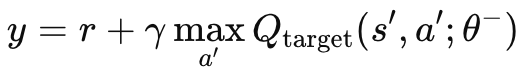
Where:

• y: The target Q-value, which represents the estimated return (future reward) starting from the current state s, taking action a, and then following the optimal policy thereafter.
• r: The immediate reward received after taking action a in state s.
• γ: The discount factor, which determines the importance of future rewards. It is a value between 0 and 1.
• max a′ Qtarget(s′,a′;θ−): The maximum predicted Q-value for the next state s′ over all possible actions a′, estimated by the target network with parameters θ−.

• Qtarget(s′,a′;θ−): The Q-value for the next state-action pair (s′,a′)(s', a')(s′,a′), predicted by the target network.
• θ−: The parameters (weights) of the target network, which are periodically updated from the main network's parameters.
• 
  

This formula is implemented in MQL5 via the critical target function, which we append to the CQL class that we had already used in our reinforcement-learning introductory article. This function is listed below:

//+------------------------------------------------------------------+
// Critic Target for DQN
//+------------------------------------------------------------------+
vector Cql::CriticTarget(vector &Rewards, vector &TargetOutput)
{  vector _target = Rewards + (THIS.gamma * TargetOutput);
   return(_target);
}

There is a bootstrapping issue. In traditional Q-learning as we saw in the prior article on reinforcement learning, the network updates the q-values based on its own predictions, which can lead to a cascade of errors (more commonly referred to as bootstrapping error) if the predictions are inaccurate. This is because the q-values for one state depend on the q-values of subsequent states, which potentially can result in error amplification.

The target network’s role therefore is to mitigate this by providing a slower-moving target. Since the target network’s parameters are updated less frequently (typically every few ten-thousand steps), it changes more gradually than the online network. This slows down the rate at which errors can propagate, thus managing the bootstrapping problem.

In situations where we have non-linear dynamics such as the complex environments of financial markets or even any other like video games, the relationships between states and rewards tends to be highly non-linear. The stability therefore introduced by the target network is critical for DQN to learn effectively in these settings. Without this target network, the online network (DQN) is more likely to diverge when faced with complex or rapidly changing environments due to the rapid updates of both q-values and targets.

In addition, the target network can be improved by adding an extension, that is often referred to as the ‘double DQN’, that addresses overestimation bias. This is implemented by using both the online and target networks separately to select and evaluate actions. It is a decoupling of the action selection and action evaluation processes between the online and target networks. The online network is used for selecting the action, while the target network evaluates it.

Experience Replay and its Role in Training

Experience replay is a buffering technique where a reinforcement-learning DQN agent stores its ‘experiences’ of state, action, reward, and next state in a replay buffer. These experiences are then sampled randomly during training to update the agent’s DQN weights and biases. This approach, is, as one would expect, useful for breaking the sequential correlation from considering only consecutive data points and could thus be more adept for real-world scenarios like the financial markets. In financial markets, consecutive data points, whether in price or contract volume, or volatility tend to be highly correlated since they are all influenced by similar market conditions and participant behaviours. Training a DQN agent on such sequentially correlated data tends to lead to overfitting and a lack of generalization, since the DQN agent gets accustomed to exploiting specific patterns that do not generalize well to different market conditions.

To break these temporal correlations, typically, the DQN is trained on mini-batches of randomly sampled experience data points from the replay buffer. The random sampling in particular helps break the temporal correlations, which results in the agent learning a better distribution of experiences which better approximate the underlying dynamics of the market. Besides better generalization, the training process over the long term becomes more stabilized and also converges better. This is because the experience replay reduces variance of updates during the training process.

Without experience replay the network weight updates would happen in bursts of highly correlated consecutive samples, only to be interrupted by a totally different update from different environment conditions, which would tend to make the whole update process very volatile potentially leading to instability in the learning process. By randomly sampling from a diverse set of experiences, the DQN agent performs smoother and more stable updates, improving convergence to an optimal policy.

The efficient utilization of historical data is something that experience-replay also enables because the agent re-learns from experience multiple times (due to the random selection) which is valuable particularly in financial markets where obtaining large amounts of diverse and representative data at any particular time is challenging. This in essence allows the DQN to learn from rare or significant events, such as market crashes or rallies, even if they are not currently happening. This makes the agent more prepared and robust for those events, should they happen.

Experience replay also enhances the exploration potential of reinforcement-learning, as opposed to just exploitation. It reduces the likelihood of ‘catastrophic forgetting’ where the agent repeatedly samples from its replay buffer, allowing it to reinforce knowledge of older strategies and preventing them from being overwritten by newer experiences; and finally, it allows even more specialized instances of experience replay like prioritized experience replay where data samples with the larger loss function errors are prioritized given their higher learning potential thus making the learning more efficient and targeted.

We mention experience replay in this article because it is a key tenet in DQN; however we will showcase its ability in MQL5 in coming articles where DQN will be more than just a hybrid loss function, but will be the primary forecasting model for our signal class.

Temporal Decision-Making

Often decisions made, even outside of trading in fields like robotics or gaming, have delayed effects on future outcomes, that are not necessarily immediate but do play out over longer time horizons. Economic news releases and company fillings is what could come to mind for traders, but this relationship establishes a temporal dependency. This temporal relationship is considered in the q-value equation above through the gamma factor. Gamma allows a balance between short-term and long-term rewards, which gives the DQN q-values the ability to look further ahead and estimate the cumulative impact of actions over time. It is argued the effect of this is that some rewards are delayed and gamma ensures that the agent does not ignore long-term rewards while still keeping tabs on the immediate ones, which can be essential when trading. For instance, often positions that are opened on major interest rate decisions, do not immediately yield favourable excursions. The adverse excursion periods usually headline these positions, and therefore the ability to have and use signals that take this into account like the DQNs can be an edge.

Changes to our prior code

To utilize our DQN within a hybrid loss function, we need to firstly append our custom loss enumeration to look as follows:

//+------------------------------------------------------------------+
//| Custom Loss-Function Enumerator                                  |
//+------------------------------------------------------------------+
enum Eloss
{  LOSS_TYPICAL = -1,
   LOSS_SVR = 1,
   LOSS_QL = 2,
   LOSS_DQN = 3
};

We add a new enumeration ‘LOSS_DQN’ to be selected when the loss function uses DQN. Additional changes we need to make as we did in the first article on reinforcement learning are in the back-propagation function, where the selection of the suitable loss type determines the value used in computing the deltas. These changes are as follows:

//+------------------------------------------------------------------+
//| BACKWARD PROPAGATION OF THE MULTI-LAYER-PERCEPTRON.              |
//+------------------------------------------------------------------+
//|                                                                  |
//| -Extra Validation check of MLP architecture settings is performed|
//|  at run-time.                                                    |
//|  Chcecking of 'validation' parameter should ideally be performed |
//|  at class instance initialisation.                               |
//|                                                                  |
//| -Run-time Validation of learning rate, decay rates and epoch     |
//|  index is performed as these are optimisable inputs.             |
//+------------------------------------------------------------------+
void Cmlp::Backward(Slearning &Learning, int EpochIndex = 1)
{  if(!validated)
   {  printf(__FUNCSIG__ + " invalid network arch! ");
      return;
   }


....

//COMPUTE DELTAS
   vector _last, _last_derivative;
   _last.Init(inputs.Size());
   if(hidden_layers == 0)
   {  _last = weights[hidden_layers].MatMul(inputs);
   }
   else if(hidden_layers > 0)
   {  _last = weights[hidden_layers].MatMul(hidden_outputs[hidden_layers - 1]);
   }
   _last.Derivative(_last_derivative, THIS.activation);
   vector _last_loss = output.LossGradient(label, THIS.loss_typical);
   if(THIS.loss_custom == LOSS_SVR)
   {  _last_loss = SVR_Loss();
   }
   else if(THIS.loss_custom == LOSS_QL)
   {  

....

   }
   else if(THIS.loss_custom == LOSS_DQN)
   {  double _reward = QL.CriticReward(Learning.ql_reward_max, Learning.ql_reward_min, Learning.ql_reward_float);
      vector _rewards;
      _rewards.Init(Learning.dqn_target.Size());
      _rewards.Fill(0.0);
      if(_reward > 0.0)
      {  _rewards[0] = 1.0;
      }
      else if(_reward == 0.0)
      {  _rewards[1] = 1.0;
      }
      else if(_reward < 0.0)
      {  _rewards[2] = 1.0;
      }
      vector _target = QL.CriticTarget(_rewards, Learning.dqn_target);
      _last_loss = output.LossGradient(_target, THIS.loss_typical);
   }
   
....


}

The other main changes we made to the code are in the CQL class and have already been highlighted above, where the q-value formula for DQN is introduced. The get output function we use for generating the condition thresholds is not very different from what we considered in the earlier article on basic q-learning. It is presented below:

//+------------------------------------------------------------------+
//|                                                                  |
//+------------------------------------------------------------------+
void CSignalDQN::GetOutput(int &Output)
{  m_learning.rate = m_learning_rate;
   for(int i = m_epochs; i >= 1; i--)
   {  MLP.LearningType(m_learning, i);
      for(int ii = m_train_set; ii >= 0; ii--)
      {  int _states = 2;
         vector _in, _in_old, _in_row, _in_row_old, _in_col, _in_col_old;
         if
         (
            _in_row.Init(_states) &&
            _in_row.CopyRates(m_symbol.Name(), m_period, 8, ii + 1, _states) &&
            _in_row.Size() == _states
            &&
            _in_row_old.Init(_states) &&
            _in_row_old.CopyRates(m_symbol.Name(), m_period, 8, ii + 1 + 1, _states) &&
            _in_row_old.Size() == _states
            &&
            _in_col.Init(_states) &&
            _in_col.CopyRates(m_symbol.Name(), m_period, 8, ii + 1, _states) &&
            _in_col.Size() == _states
            &&
            _in_col_old.Init(_states) &&
            _in_col_old.CopyRates(m_symbol.Name(), m_period, 8, m_state_lag + ii + 1, _states) &&
            _in_col_old.Size() == _states
         )
         {  _in_row -= _in_row_old;
            _in_col -= _in_col_old;
            //
            m_learning.ql_reward_max = _in_row.Max();
            m_learning.ql_reward_min = _in_row.Min();
            if(m_learning.ql_reward_max == m_learning.ql_reward_min)
            {  m_learning.ql_reward_max += m_symbol.Point();
            }
            MLP.Set(_in_row);
            MLP.Forward();
            //
            MLP.QL.THIS.environments = m_environments;
            //
            vector _in_e;
            _in_e.Init(1);
            MLP.QL.Environment(_in_row, _in_col, _in_e);
            //
            int _row = 0, _col = 0;
            MLP.QL.SetMarkov(int(_in_e[_states - 1]), _row, _col);
            _in.Init(2);
            _in[0] = _row;
            _in[1] = _col;
            DQN_ONLINE.Set(_in);
            DQN_ONLINE.Forward();
            //
            MLP.QL.SetMarkov(int(_in_e[_states - 2]), _row, _col);
            _in_old.Init(2);
            _in_old[0] = _row;
            _in_old[1] = _col;
            DQN_TARGET.Set(_in_old);
            DQN_TARGET.Forward();
            m_learning.dqn_target = DQN_TARGET.output;
            if(ii > 0)
            {  vector _target, _target_data, _target_data_old;
               if
               (
                  _target_data.Init(2) &&
                  _target_data.CopyRates(m_symbol.Name(), m_period, 8, ii, 2) &&
                  _target_data.Size() == 2
                  &&
                  _target_data_old.Init(2) &&
                  _target_data_old.CopyRates(m_symbol.Name(), m_period, 8, ii + 1, 2) &&
                  _target_data_old.Size() == 2
               )
               {  _target.Init(__MLP_OUTPUTS);
                  _target.Fill(0.0);
                  _target_data -= _target_data_old;
                  double _type = _target_data[1] - _in_row[1];
                  int _index = (_type < 0.0 ? 0 : (_type > 0.0 ? 2 : 1));
                  _target[_index] = 1.0;
                  MLP.Get(_target);
                  if(i == m_epochs && ii == m_train_set)
                  {  DQN_ONLINE.Backward(m_learning, i);
                     if(m_target_counter >= m_target_counts)
                     {  DQN_TARGET = DQN_ONLINE;
                        m_target_counter = 0;
                     }
                     MLP.Backward(m_learning, i);
                  }
               }
            }
            Output = (MLP.output.Max()==MLP.output[0]?0:(MLP.output.Max()==MLP.output[1]?1:2));
         }
      }
   }
}

As mentioned already above, we have 2 DQN networks, the online network and the target network. In addition, of course, is the parent MLP which takes close price changes as inputs, like in the q-learning article. We should not be referring to the QL class, besides calling the critical target function to get DQN’s q-values as mentioned above. However, because the QL class allows us to access the environment state coordinates (when given an index) as well as composing as index from state coordinates, we are referring to it to get the inputs for the two DQN networks. As mentioned, we are not using the q-map for our forecasts but are relying on the online DQN network which is trained by the target network. Both the online and target DQNs simply take environment states (old and new, respectively) and are trained to forecast a vector of q values (for each agent action).

Strategy Tester Reports:

We test this MLP with reinforcement-learning training via Deep-Q-networks on EURGBP for the year 2023 on the daily time frame. Below are our results, which are meant to strictly demonstrate tradability and not necessarily replication on future market action.

Conclusion

We have looked at the implementation and testing of an alternative algorithm to reinforcement-learning called Deep-Q-Networks in wizard assembled Expert Advisors. Reinforcement-learning is the 3^rd method at training in machine learning besides supervised learning and unsupervised learning and although it is strictly speaking a different approach at training within machine learning, in subsequent articles we will consider scenarios where it can actually serve as the primary model and signal generator.