Data Science and ML(Part 30): The Power Couple for Predicting the Stock Market, Convolutional Neural Networks(CNNs) and Recurrent Neural Networks(RNNs)

Contents

• Introduction
• Understanding RNNs and CNNs
• The synergy of CNNs and RNNs
• Feature extraction with CNNs
• Temporal modeling with RNNs
• Training and making predictions
• A combination of CNN and LSTM
• A combination of CNN and GRU
• Conclusion

Introduction

In the previous articles, we have seen how powerful both Convolutional Neural Networks (CNNs) and Recurrent Neural Networks (RNNs) are and how they can be deployed to help beat the market by providing us with valuable trading signals.

In this one we are going to attempt combining two of the most powerful techniques CNN and RNN and observe their predictive impact in the stock market. But before that let us briefly understand what CNN and RNN are all about.

Understanding Recurrent Neural Networks (RNNs) and Convolutional Neural Networks (CNNs)

Convolutional Neural Networks (CNNs), are designed to recognize patterns and features in the data, despite originally being developed for image recognition tasks, they perform well in tabular data that is specifically designed for time series forecasting.

As said in the previous articles, they operate by firstly applying filters to the input data then they extract high-level features that can be useful for prediction. In stock market data, these features include trends, seasonal effects, and anomalies.

CNN architecture

By leveraging the hierarchical nature of CNNs, we can uncover layers of data representations, each providing insights into different aspects of the market.

Recurrent Neural Networks (RNNs) are artificial neural networks designed to recognize patterns in sequences of data, such as time series, languages, or in videos.

Unlike traditional neural networks, which assume that inputs are independent of each other, RNNs can detect and understand patterns from a sequence of data (information).

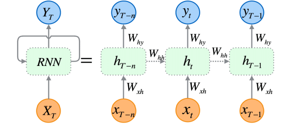
RNNs are explicitly designed for sequential data, Their architecture allows them to maintain a memory of previous inputs, making them very suitable for time series forecasting since are capable of understanding temporal dependencies within the data which is crucial for making accurate predictions in the stock market.

As I explained in part 25 of this article series, There are three (commonly used) specific types of RNNs which include, a vanilla Recurrent Neural Network(RNN), Long-Short Term Memory(LSTM), and Gated Recurrent Unit(GRU).

Since CNNs excel at extracting and detecting features from the data, RNNs are exceptional at interpreting these features over time. The idea is simple, to combine these two and see if we can build a powerful and robust model capable of making better predictions in the stock market.

The Synergy of CNNs and RNNs

To integrate these two, we are going to create the models in three steps.

1. Feature Extraction with CNNs
   
2. Temporal Modeling with RNNs
   
3. Training and Getting Predictions
   

Let us go through one step after the other and build this robust model comprised of both RNN and LSTM.

01: Feature Extraction with CNNs

This first step involves feeding the time series data into a CNN model, the CNN model processes the data, identifying significant patterns and extracting relevant features. 

Using the Tesla stock dataset which consists of Open, High, Low, and Close values. Let us start by preparing the data into a 3D time series format acceptable by CNNs and RNNs.

Let us create the target variable for a classification problem.

Python code

target_var = []

open_price = new_df["Open"] 
close_price = new_df["Close"]

for i in range(len(open_price)): 
    if close_price[i] > open_price[i]: # Closing price is greater than opening price
        target_var.append(1) # buy signal
    else:
        target_var.append(0) # sell signal

We normalize the data using the Standard scaler to make it robust for ML purposes.

X = new_df.iloc[:, :-1]
y = target_var

# Scalling the data

scaler = StandardScaler()
X = scaler.fit_transform(X)

# Train-test split

X_train, X_test, y_train, y_test = train_test_split(X, y, test_size=0.2, shuffle=False)

print(f"x_train = {X_train.shape} - x_test = {X_test.shape}\n\ny_train = {len(y_train)} - y_test = {len(y_test)}")

 Outputs

x_train = (799, 3) - x_test = (200, 3)

y_train = 799 - y_test = 200

We can then prepare the data into time series format.

# creating the sequence 

X_train, y_train = create_sequences(X_train, y_train, time_step)
X_test, y_test = create_sequences(X_test, y_test, time_step)

Since this is a classification problem, we one-hot encode the target variable.

from tensorflow.keras.utils import to_categorical

y_train_encoded = to_categorical(y_train)
y_test_encoded = to_categorical(y_test)

print(f"One hot encoded\n\ny_train {y_train_encoded.shape}\ny_test {y_test_encoded.shape}")

Outputs

One hot encoded

y_train (794, 2)
y_test (195, 2)

Feature extraction is performed by the CNN model itself, Let's give the model raw data we just prepared it.

model = Sequential()
model.add(Conv1D(filters=16, 
                 kernel_size=3, 
                 activation='relu', 
                 strides=2,
                 padding='causal',
                 input_shape=(time_step, X_train.shape[2])
                )
         )

model.add(MaxPooling1D(pool_size=2))

02: Temporal Modeling with RNNs

The extracted features in the previous step are then passed to the RNN model. The model processes these features, considering the temporal order and dependencies within the data.

Unlike the CNN model architecture we used in part 27 of this article series where we used Fully Connected Neural Network Layers right after the Flatten layer. This time we replace these regular Neural Network(NN) layers with Recurrent Neural Network (RNN) layers.

Without forgetting to remove the "Flatten layer" that is seen in the CNN architecture image.

We remove the Flatten layer in the CNN architecture because this layer is typically used to convert a 3D input into a 2D output meanwhile the RNNs (RNN, LSTM, and GRU) expects a 3D input data in the form of (batch size, time steps, features).

model.add(MaxPooling1D(pool_size=2))

model.add(SimpleRNN(50, activation='relu'))
model.add(Dropout(0.5))
model.add(Dense(50, activation='relu'))
model.add(Dropout(0.5))
model.add(Dense(units=len(np.unique(y)), activation='softmax'))  # Softmax for binary classification (1 buy, 0 sell signal)

03: Training and Getting Predictions

Finally, we can proceed to train the model we built in the prior two steps, after that, we validate it, measure its performance then get the predictions out of it.

Python code

model.summary()

# Compile the model
optimizer = Adam(learning_rate=0.0001)
model.compile(optimizer=optimizer, loss='binary_crossentropy', metrics=['accuracy'])

# Train the model
early_stopping = EarlyStopping(monitor='val_loss', patience=10, restore_best_weights=True)

history = model.fit(X_train, y_train_encoded, epochs=1000, batch_size=16, validation_split=0.2, callbacks=[early_stopping])

plt.figure(figsize=(7.5, 6))
plt.plot(history.history['loss'], label='Training Loss')
plt.plot(history.history['val_loss'], label='Validation Loss')
plt.xlabel('Epochs')
plt.ylabel('Loss')
plt.title('Training Loss Curve')
plt.legend()
plt.savefig("training loss curve-rnn-cnn-clf.png")
plt.show()

# Evaluating the Trained Model

y_pred = model.predict(X_test) 


classes_in_y = np.unique(y)
y_pred_binary = classes_in_y[np.argmax(y_pred, axis=1)]

# Confusion Matrix
cm = confusion_matrix(y_test, y_pred_binary)
sns.heatmap(cm, annot=True, fmt='d', cmap='Blues')
plt.xlabel("Predicted Label")
plt.ylabel("True Label")
plt.title("Confusion Matrix")
plt.savefig("confusion-matrix RNN + CNN.png")  # Display the heatmap


print("Classification Report\n",
      classification_report(y_test, y_pred_binary))

Outputs

After evaluating the model after 14 epochs, The model was 54% accurate on the test data.

7/7 ━━━━━━━━━━━━━━━━━━━━ 0s 33ms/step
Classification Report
               precision    recall  f1-score   support

           0       0.70      0.40      0.51       117
           1       0.45      0.74      0.56        78

    accuracy                           0.54       195
   macro avg       0.58      0.57      0.54       195
weighted avg       0.60      0.54      0.53       195

It is worth mentioning that training the final model did take some time when more layers were added, this is due to the complex nature of the two models we combined. 

After training, I had to save the final model to ONNX format.

Python code

onnx_file_name = "rnn+cnn.TSLA.D1.onnx"

spec = (tf.TensorSpec((None, time_step, X_train.shape[2]), tf.float16, name="input"),)
model.output_names = ['outputs']

onnx_model, _ = tf2onnx.convert.from_keras(model, input_signature=spec, opset=13)

# Save the ONNX model to a file
with open(onnx_file_name, "wb") as f:
    f.write(onnx_model.SerializeToString())

Without forgetting to save the Standardization scaler parameters too.

# Save the mean and scale parameters to binary files

scaler.mean_.tofile(f"{onnx_file_name.replace('.onnx','')}.standard_scaler_mean.bin")
scaler.scale_.tofile(f"{onnx_file_name.replace('.onnx','')}.standard_scaler_scale.bin")

I opened the saved ONNX model in Netron, It is a massive one.

Similar to how we deployed the Convolutional Neural Network (CNN) before, We can use the same library to aid us with the task of reading this massive model effortlessly in MQL5.

#include <MALE5\Convolutional Neural Networks(CNNs)\ConvNet.mqh>
#include <MALE5\preprocessing.mqh>

CConvNet cnn;
StandardizationScaler *scaler; //from preprocessing.mqh

But, before that, we have to add the ONNX model and Standardization scaler parameters to our Expert Advisor as resources.

#resource "\\Files\\rnn+cnn.TSLA.D1.onnx" as uchar onnx_model[]
#resource "\\Files\\rnn+cnn.TSLA.D1.standard_scaler_mean.bin" as double standardization_mean[]
#resource "\\Files\\rnn+cnn.TSLA.D1.standard_scaler_scale.bin" as double standardization_std[]

The first thing we have to do inside the OnInit function is to initialize them both (the standardization scaler and the CNN model).

int OnInit()
  {
//---
   
   if (!cnn.Init(onnx_model)) //Initialize the Convolutional neural network 
     return INIT_FAILED;
   
   scaler = new StandardizationScaler(standardization_mean, standardization_std); //Initialize the saved scaler by populating it with values 
  
   ...
   ...
        
  return (INIT_SUCCEEDED);       
 }

To get the predictions, we have to normalize the input data using this preloaded scaler, then we apply the normalized data to the CNN model and get the predicted signal and probabilities.

   if (NewBar()) //Trade at the opening of a new candle
    {
      CopyRates(Symbol(), PERIOD_D1, 1, time_step, rates);
      
      for (ulong i=0;  i<x_data.Rows(); i++)
        {
          x_data[i][0] = rates[i].open;
          x_data[i][1] = rates[i].high;
          x_data[i][2] = rates[i].low;
        }
   
   //---
            
      x_data = scaler.transform(x_data); //Normalize the data
       
      int signal = cnn.predict_bin(x_data, classes_in_data_); //getting a trading signal from the RNN model
      vector probabilities = cnn.predict_proba(x_data);  //probability for each class
     
      Comment("Probability = ",probabilities,"\nSignal = ",signal);

Below is how the comment looks on the chart.

The probability vector depends on the classes that were present in the target variable of your training data. From the training data, we prepared the target variable to indicate 0 for a sell signal and 1 for a buy signal. The class identifiers or numbers must be in ascending order.

input int time_step = 5; 
input int magic_number = 24092024;
input int slippage = 100;

MqlRates rates[];
matrix x_data(time_step, 3); //3 columns for open, high and low
vector classes_in_data_ = {0, 1}; //unique target variables as they are in the target variable in your training data
int OldNumBars = 0;
//+------------------------------------------------------------------+
//| Expert initialization function                                   |
//+------------------------------------------------------------------+
int OnInit()
  {
//---

The matrix named x_data is the one responsible for the temporary storage of independent variables (features) from the market. This matrix is resized to 3 columns since we trained the model on 3 features (Open, High, and Low), and resized to the number of rows equal to the time step value.

The time step value must be similar to the one used in creating sequential training data.

We can make a simple strategy based on signals provided by the model we built.

   double min_lot = SymbolInfoDouble(Symbol(), SYMBOL_VOLUME_MIN);
     
      MqlTick ticks;
      SymbolInfoTick(Symbol(), ticks);
      
      if (signal==1) //if the signal is bullish
       {    
          ClosePos(POSITION_TYPE_SELL); //close sell trades when the signal is buy
          
          if (!PosExists(POSITION_TYPE_BUY)) //There are no buy positions
           {
             if (!m_trade.Buy(min_lot, Symbol(), ticks.ask, 0 , 0)) //Open a buy trade
               printf("Failed to open a buy position err=%d",GetLastError());
           }
       }
      else if (signal==0) //Bearish signal
        {
          ClosePos(POSITION_TYPE_BUY); //close all buy trades when the signal is sell
          
          if (!PosExists(POSITION_TYPE_SELL)) //There are no Sell positions
           {
            if (!m_trade.Sell(min_lot, Symbol(), ticks.bid, 0 , 0)) //open a sell trade
               printf("Failed to open a sell position err=%d",GetLastError());
           }
        }
      else //There was an error
        return;

Now that we have the model loaded up and ready to make predictions, I ran a test from 2020.01.01 to 2024.09.01. Below is the full tester configuration (settings) image.

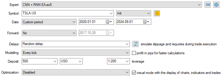
Notice I applied the EA on a 4-Hour chart, Instead of the Daily timeframe which the Tesla stock data was collected from. This is because we programmed the strategy and models to kick into action an instant after the new candle is opened but, the daily candle is usually opened when the market is closed hence causing the EA to miss on trading until the next day. 

By applying the EA to a lower timeframe (4-Hour timeframe in this case) we ensure that we continuously monitor the market after every 4 hours and perform some trading activities. 

This doesn't affect the data provided to the EA as we applied the CopyRates function to the daily timeframe (trading decisions still depend on the daily chart)

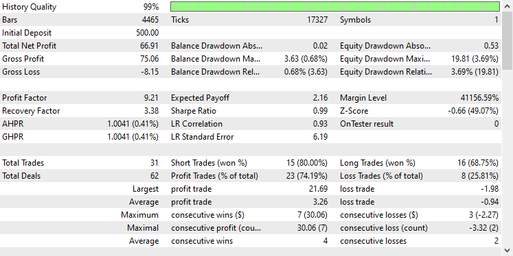
Below is the Tester's outcome.

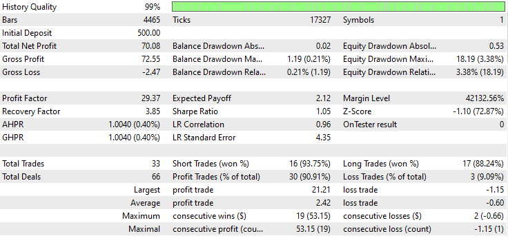
Impressive! The EA produced 90% profitable trades. The AI model was just a Simple RNN.

Now let's see how well LSTM and GRU perform in the same market.

A combination of Convolutional Neural Network (CNN) and Long-Short Term Memory (LSTM)

Unlike the simple RNN which is incapable when it comes to understanding patterns within long sequences of data or information, the LSTM can understand relationships and patterns in long sequences of information.

LSTMs are often more efficient and accurate than simple RNNs. Let us create a CNN model with LSTM in it and then observe how it fares in the Tesla stock.

Python code

from tensorflow.keras.layers import LSTM

# Define the CNN model

model = Sequential()
model.add(Conv1D(filters=16, 
                 kernel_size=3, 
                 activation='relu', 
                 strides=2,
                 padding='causal',
                 input_shape=(time_step, X_train.shape[2])
                )
         )

model.add(MaxPooling1D(pool_size=2))


model.add(LSTM(50, activation='relu'))
model.add(Dropout(0.5))
model.add(Dense(50, activation='relu'))
model.add(Dropout(0.5))
model.add(Dense(units=len(np.unique(y)), activation='softmax'))  # For binary classification (e.g., buy/sell signal)

model.summary()

Since all RNNs can be implemented the same way, I had to make only one change in the block of code used to create a simple RNN.

After training and validating the model, its accuracy was 53% on the testing data.

7/7 ━━━━━━━━━━━━━━━━━━━━ 0s 36ms/step
Classification Report
               precision    recall  f1-score   support

           0       0.67      0.44      0.53       117
           1       0.45      0.68      0.54        78

    accuracy                           0.53       195
   macro avg       0.56      0.56      0.53       195
weighted avg       0.58      0.53      0.53       195

In the MQL5 programming language, we can use the same library we used for the simple RNN EA.

#resource "\\Files\\lstm+cnn.TSLA.D1.onnx" as uchar onnx_model[]
#resource "\\Files\\lstm+cnn.TSLA.D1.standard_scaler_mean.bin" as double standardization_mean[]
#resource "\\Files\\lstm+cnn.TSLA.D1.standard_scaler_scale.bin" as double standardization_std[]

#include <MALE5\Convolutional Neural Networks(CNNs)\ConvNet.mqh>
#include <MALE5\preprocessing.mqh>

CConvNet cnn;
StandardizationScaler *scaler;

The rest of the code is kept the same as in the CNN + RNN EA.

I used the same Tester's settings as before, below was the outcome.

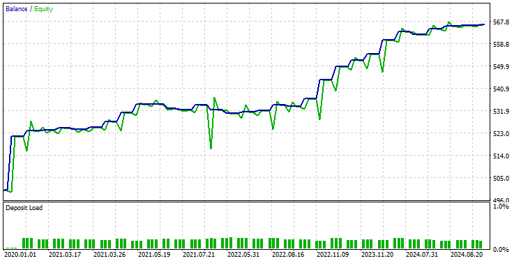
This time the overall trades accuracy is approximately 74%, It is lower than what we got in the previous model but, still outstanding!

A combination of Convolutional Neural Network (CNN) and Gated Recurrent Unit (GRU)

Just like the LSTM, GRU models are also capable of understanding the relationships between long sequences of information and data despite having a minimalist approach compared to that of the LSTM model.

We can implement it the same as other RNN models, we only make the change in the type of model in the code for building the CNN model architecture.

from tensorflow.keras.layers import GRU

# Define the CNN model

model = Sequential()
model.add(Conv1D(filters=16, 
                 kernel_size=3, 
                 activation='relu', 
                 strides=2,
                 padding='causal',
                 input_shape=(time_step, X_train.shape[2])
                )
         )

model.add(MaxPooling1D(pool_size=2))


model.add(GRU(50, activation='relu'))
model.add(Dropout(0.5))
model.add(Dense(50, activation='relu'))
model.add(Dropout(0.5))
model.add(Dense(units=len(np.unique(y)), activation='softmax'))  # For binary classification (e.g., buy/sell signal)

model.summary()

After training and validating the model, the model achieved an accuracy similar to that of LSTM, 53% accuracy on the testing data.

7/7 ━━━━━━━━━━━━━━━━━━━━ 1s 41ms/step
Classification Report
               precision    recall  f1-score   support

           0       0.69      0.39      0.50       117
           1       0.45      0.73      0.55        78

    accuracy                           0.53       195
   macro avg       0.57      0.56      0.53       195
weighted avg       0.59      0.53      0.52       195

We load the GRU model in ONNX format and its scaler parameters in binary files.

#resource "\\Files\\gru+cnn.TSLA.D1.onnx" as uchar onnx_model[]
#resource "\\Files\\gru+cnn.TSLA.D1.standard_scaler_mean.bin" as double standardization_mean[]
#resource "\\Files\\gru+cnn.TSLA.D1.standard_scaler_scale.bin" as double standardization_std[]

#include <MALE5\Convolutional Neural Networks(CNNs)\ConvNet.mqh>
#include <MALE5\preprocessing.mqh>

CConvNet cnn;
StandardizationScaler *scaler;

Again the rest of the code is the same as the one used in the simple RNN EA.

After testing the model on the Tester using the same settings, below was the outcome.

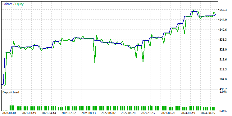
The GRU model provided an accuracy of approximately 61%, not as good as the prior two models but, a decent accuracy indeed.

Final Thoughts

The integration of Convolutional Neural Networks (CNNs) with Recurrent Neural Networks (RNNs) can be a powerful approach to stock market prediction, offering the potential to uncover hidden patterns and temporal dependencies in data. However, this combination is relatively uncommon and comes with certain challenges. One of the key risks is overfitting, especially when applying such sophisticated models to relatively simple problems. Overfitting can cause the model to perform well on training data but fail to generalize to new data.

Additionally, the complexity of combining CNNs and RNNs leads to significant computational costs, particularly if you decide to scale up the model by adding more dense layers or increasing the number of neurons. It is essential to carefully balance model complexity with the resources available and the problem at hand.

Peace out.

Track development of machine learning models and much more discussed in this article series on this GitHub repo.

Attachments Table

File name	File type	Description & Usage
Experts\CNN + GRU EA.mq5 Experts\CNN + LSTM EA.mq5 Experts\CNN + RNN EA.mq5	Expert Advisors	Trading robot for loading the ONNX models and testing the trading strategy in MetaTrader 5.
ConvNet.mqh preprocessing.mqh	Include files	- This file comprises code for loading CNN models saved in ONNX format. - The Standardization scaler can be found in this file
Files\ *.onnx	ONNX models	Machine learning models discussed in this article in ONNX format
Files\*.bin	Binary files	Binary files for loading Standardization scaler parameters for each model
Jupyter Notebook\cnns-rnns.ipynb	python/Jupyter notebook	All the Python code discussed in this article can be found inside this notebook.