Data Science and Machine Learning (Part 21): Unlocking Neural Networks, Optimization algorithms demystified

MetaTrader 5 — Tester | 22 March 2024, 09:47

4 728

I’m not suggesting that neural networks are easy. You need to be an expert to make these things work. But that expertise serves you across a broader spectrum of applications. In a sense, all of the efforts that previously went into feature design now goes into architecture design loss function design, and optimization scheme design. The manual labor has been raised to a higher level of abstraction.

Stefano Soatto

Introduction

It seems like everybody nowadays is interested in Artificial Intelligence, it's everywhere, and the big guys in the tech industry such as Google and Microsoft behind openAI are pushing for AI adaptation in different aspects and industries such as entertainment, healthcare industry, arts, creativity, etc.

I see this trend also in the MQL5 community why not, with the introduction of matrices and vectors and ONNX to MetaTrader5. It is now possible to make Artificial intelligence trading models of any complexity. You don't even need to be an expert in Linear algebra or a nerd enough to understand everything that goes into the system.

Despite all that, the fundamentals of machine learning are now more difficult to find than ever, yet they are as important knowing to solidify your understanding of AI. They let you know why you do what you do which makes you flexible and lets you exercise your options. There is a lot of things we are yet to discuss on machine learning. Today we'll see what are the optimization algorithms, how they fare against one another, when and which optimization algorithm you should choose for a better performance and accuracy to your Neural networks.

The content discussed in this article will help you understand optimization algorithms in general, meaning this knowledge will serve you even while working with Scikit-Learn, Tensorflow, or Pytorch models from Python, as these optimizers are universal for all neural networks no matter which programming language you use.

What are the Neural Network Optimizers?

By definition, optimizers are algorithms that fine-tune neural network parameters during training. Their goal is to minimize the loss function, ultimately leading to enhanced performance.

Simply put, neural network optimizers do:

These are the key parameters that influence the neural network. Optimizers determine how to modify each parameter in each training iteration.
Optimizers gauge the discrepancy between actual values and neural network predictions. They strive to reduce this error progressively.

I recommend reading a prior article Neural Networks Demystified if you haven't already. In this article we will be improving the neural network model we built from scratch in this article, adding the optimizers to it.

Before we see what are different types of optimizers are, we need to understand the algorithms for backpropagation. There are commonly three algorithms;

Stochastic Gradient Descent(SGD)
Batch Gradient Descent(BGD)
Mini-Batch Gradient Descent

01: Stochastic Gradient Descent Algorithm(SGD)

Stochastic Gradient Descent (SGD), is a fundamental optimization algorithm used to train neural networks. It iteratively updates the weights and biases of the network in a way that minimizes the loss function. The loss function measures the discrepancy between the network's predictions and the actual labels (target values) in the training data.

The main processes involved in these optimization algorithms are the same, they include;

iteration
backpropagation
weights and bias update

These algorithms differ in how iterations are handled and how often the weights and biases are updated. The SGD algorithm updates neural network parameters(weights and biases) one training example(data point) at a time.

void CRegressorNets::backpropagation(const matrix& x, const vector &y)
 {   
    for (ulong epoch=0; epoch<epochs && !IsStopped(); epoch++)
      { 
        
        for (ulong iter=0; iter<rows; iter++) //iterate through all data points
          {             
             for (int layer=(int)mlp.hidden_layers-1; layer>=0 && !IsStopped(); layer--) //Loop through the network backward from last to first layer
               {    
                // find partial derivatives of each layer WRT the loss function dW and dB
                
                 
                //--- Weights updates
                 
                 optimizer_weights.update(W, dW);
                 optimizer_bias.update(B, dB);
                 
                 this.W_tensor.Add(W, layer);
                 this.B_tensor.Add(B, layer);
               }
         }
     }
 }

Its Advantages:

Computationally efficient for large datasets.
Can sometimes converge faster than BGD and Mini-batch gradient descent, especially for non-convex loss functions as it uses one training sample at a time.
Good at avoiding the local minima: Due to the noisy updates in SGD, it has the ability to escape from local minima and converge to global minima.

Disadvantages:

Updates can be noisy, leading to zig-zagging behavior during training.
May not always converge to the global minimum.
Slow convergence, may require more epochs to convergence since it updates the parameters for each training example one at a time.
Sensitive to the learning rate: The choice of learning rate can be critical to this algorithm, a higher learning rate may cause the algorithm to overshoot the global minima, while lower learning rate slows the convergence process.

Stochastic gradient descent is more suitable for optimizing non-convex functions since it can escape local minima and find the global minimum.

02: Batch Gradient Descent Algorithm(BGD):

Unlike SGD, Batch gradient Descent(BGD) calculates gradients using the entire dataset in each iteration.

Advantages:

In theory, converges to a minimum if the loss function is smooth and convex.

Disadvantages:

Can be computationally expensive for large datasets, as it requires processing the entire dataset repeatedly.

I will not implement it in the neural network we have at the moment, but can be implemented easily just like the Mini-batch gradient descent below, you can implement it if you'd like.

03: Mini-Batch Gradient Descent:

This algorithm is a compromise between SGD and BGD, it updates the network's parameters using a small subset (mini-batch) of the training data in each iteration.

Advantages:

Provides a good balance between computational efficiency and update stability compared to SGD and BGD.
Can handle larger datasets more effectively than BGD.

Disadvantages:

May require more tuning of the mini-batch size compared to SGD.
Computationally expensive compared to SGD, consumes a lot of memory for batch storing and processing.
Can take a long time to train for many large batches.

Below is the pseudocode of how Mini-batch gradient descent algorithm looks like:

void CRegressorNets::backpropagation(const matrix& x, const vector &y, OptimizerSGD *sgd, const uint epochs, uint batch_size=0, bool show_batch_progress=false)
 {

  //....
    for (ulong epoch=0; epoch<epochs && !IsStopped(); epoch++)
      { 
               
            for (uint batch=0, batch_start=0, batch_end=batch_size; batch<num_batches; batch++, batch_start+=batch_size, batch_end=(batch_start+batch_size-1))
               {
                  matrix batch_x = MatrixExtend::Get(x, batch_start, batch_end-1);
                  vector batch_y = MatrixExtend::Get(y, batch_start, batch_end-1);
                  
                  rows = batch_x.Rows();              
                  
                    for (ulong iter=0; iter<rows ; iter++) //replace to rows 
                      {
                        pred_v[0] = predict(batch_x.Row(iter));
                        actual_v[0] = y[iter];
                        
                        // Find derivatives WRT weights dW and bias dB    
                        //....                    
                            
                         //--- Updating the weights using a given optimizer
                           
                           optimizer_weights.update(W, dW); 
                           optimizer_bias.update(B, dB);
                           
                           this.Weights_tensor.Add(W, layer);
                           this.Bias_tensor.Add(B, layer);  
                        }
                   }
       }
 }

In the heart of these two algorithms by default, they have a simple gradient descent update rule, which is often referred to as SGD or Mini-BGD optimizer.

class OptimizerSGD
  {
protected:
   double m_learning_rate;
   
public:
                     OptimizerSGD(double learning_rate=0.01);
                    ~OptimizerSGD(void);
                     
                    virtual void update(matrix &parameters, matrix &gradients);
  };
//+------------------------------------------------------------------+
//|                                                                  |
//+------------------------------------------------------------------+
OptimizerSGD::OptimizerSGD(double learning_rate=0.01):
 m_learning_rate(learning_rate)
 {
 
 }
//+------------------------------------------------------------------+
//|                                                                  |
//+------------------------------------------------------------------+
OptimizerSGD::~OptimizerSGD(void)
 {
 
 }
//+------------------------------------------------------------------+
//|                                                                  |
//+------------------------------------------------------------------+
void OptimizerSGD::update(matrix &parameters, matrix &gradients)
 {
    parameters -= this.m_learning_rate * gradients; //Simple gradient descent update rule
 }
 
 
//+------------------------------------------------------------------+
//|  Batch Gradient Descent (BGD): This optimizer computes the       |
//|  gradients of the loss function on the entire training dataset   |
//|  and updates the parameters accordingly. It can be slow and      |
//|  memory-intensive for large datasets but tends to provide a      |
//|  stable convergence.                                             |
//+------------------------------------------------------------------+


class OptimizerMinBGD: public OptimizerSGD
  {
public:
                     OptimizerMinBGD(double learning_rate=0.01);
                    ~OptimizerMinBGD(void);
  };
//+------------------------------------------------------------------+
//|                                                                  |
//+------------------------------------------------------------------+
OptimizerMinBGD::OptimizerMinBGD(double learning_rate=0.010000): OptimizerSGD(learning_rate)
 {
 
 }
//+------------------------------------------------------------------+
//|                                                                  |
//+------------------------------------------------------------------+
OptimizerMinBGD::~OptimizerMinBGD(void)
 {
 
 }

Now let's train a model using these two optimizers and observe the outcome just to understand them better:

#include <MALE5\MatrixExtend.mqh>
#include <MALE5\preprocessing.mqh>
#include <MALE5\metrics.mqh>
#include <MALE5\Neural Networks\Regressor Nets.mqh>
CRegressorNets *nn;


StandardizationScaler scaler;
vector open_, high_, low_;

vector hidden_layers = {5};
input uint nn_epochs = 100;
input double nn_learning_rate = 0.0001;
input uint nn_batch_size =32;
input bool show_batch = false;
//+------------------------------------------------------------------+
//| Script program start function                                    |
//+------------------------------------------------------------------+
void OnStart()
  {
//---

  string headers;
  matrix dataset = MatrixExtend::ReadCsv("airfoil_noise_data.csv", headers);
  
  matrix x_train, x_test;
  vector y_train, y_test;
  
  MatrixExtend::TrainTestSplitMatrices(dataset, x_train, y_train, x_test, y_test, 0.7);
  
  nn = new CRegressorNets(hidden_layers, AF_RELU_, LOSS_MSE_); 
  
  x_train = scaler.fit_transform(x_train);
  
  nn.fit(x_train, y_train, new OptimizerMinBGD(nn_learning_rate), nn_epochs, nn_batch_size, show_batch);
   
  delete nn; 
  }

When nn_batch_size input is assigned a value greater than zero, the Mini-Batch gradient descent will be activated no matter which Optimizer is applied to the fit/backpropagation function.

backprop CRegressorNets::backpropagation(const matrix& x, const vector &y, OptimizerSGD *optimizer, const uint epochs, uint batch_size=0, bool show_batch_progress=false)
 {
//...
//...

//--- Optimizer use selected optimizer when batch_size ==0 otherwise use the batch gradient descent
      
   OptimizerSGD optimizer_weights = optimizer;
   OptimizerSGD optimizer_bias = optimizer;
   
   if (batch_size>0)
    {
      OptimizerMinBGD optimizer_weights;
      OptimizerMinBGD optimizer_bias;
    }
     
//--- Cross validation

    CCrossValidation cross_validation;      
    CTensors *cv_tensor;
    matrix validation_data = MatrixExtend::concatenate(x, y);
    matrix validation_x;
    vector validation_y;
    
    cv_tensor = cross_validation.KFoldCV(validation_data, 10); //k-fold cross validation | 10 folds selected
    
//---

    matrix DELTA = {};
    double actual=0, pred=0;
    
    matrix temp_inputs ={};
    
    matrix dB = {}; //Bias Derivatives
    matrix dW = {}; //Weight Derivatives
    
   
    for (ulong epoch=0; epoch<epochs && !IsStopped(); epoch++)
      {        
        double epoch_start = GetTickCount(); 

        uint num_batches = (uint)MathFloor(x.Rows()/(batch_size+DBL_EPSILON));
        
        vector batch_loss(num_batches), 
               batch_accuracy(num_batches);
                       
         vector actual_v(1), pred_v(1), LossGradient = {};
         if (batch_size==0) //Stochastic Gradient Descent
          {
           for (ulong iter=0; iter<rows; iter++) //iterate through all data points
             {
               pred = predict(x.Row(iter));
               actual = y[iter];
               
               pred_v[0] = pred; 
               actual_v[0] = actual; 
   //---
                
                DELTA.Resize(mlp.outputs,1);
                
                for (int layer=(int)mlp.hidden_layers-1; layer>=0 && !IsStopped(); layer--) //Loop through the network backward from last to first layer
                  {    
                    //..... backpropagation and finding derivatives code        
                    
                    //-- Observation | DeLTA matrix is same size as the bias matrix
                    
                    W = this.Weights_tensor.Get(layer);
                    B = this.Bias_tensor.Get(layer);
                  
                   //--- Derivatives wrt weights and bias
                  
                    dB = DELTA;
                    dW = DELTA.MatMul(temp_inputs.Transpose());                   
                    
                   //--- Weights updates
                    
                    optimizer_weights.update(W, dW);
                    optimizer_bias.update(B, dB);
                    
                    this.Weights_tensor.Add(W, layer);
                    this.Bias_tensor.Add(B, layer);
                  }
             }
         }
        else //Batch Gradient Descent
          {
               
            for (uint batch=0, batch_start=0, batch_end=batch_size; batch<num_batches; batch++, batch_start+=batch_size, batch_end=(batch_start+batch_size-1))
               {
                  matrix batch_x = MatrixExtend::Get(x, batch_start, batch_end-1);
                  vector batch_y = MatrixExtend::Get(y, batch_start, batch_end-1);
                  
                  rows = batch_x.Rows();              
                  
                    for (ulong iter=0; iter<rows ; iter++) //iterate through all data points
                      {
                        pred_v[0] = predict(batch_x.Row(iter));
                        actual_v[0] = y[iter];
                        
            //---
                        
                      DELTA.Resize(mlp.outputs,1);
                      
                      for (int layer=(int)mlp.hidden_layers-1; layer>=0 && !IsStopped(); layer--) //Loop through the network backward from last to first layer
                        {    
                         //..... backpropagation and finding derivatives code   
                            }
                          
                          //-- Observation | DeLTA matrix is same size as the bias matrix
                          
                          W = this.Weights_tensor.Get(layer);
                          B = this.Bias_tensor.Get(layer);
                        
                         //--- Derivatives wrt weights and bias
                        
                          dB = DELTA;
                          dW = DELTA.MatMul(temp_inputs.Transpose());                   
                          
                         //--- Weights updates
                          
                          optimizer_weights.update(W, dW);
                          optimizer_bias.update(B, dB);
                          
                          this.Weights_tensor.Add(W, layer);
                          this.Bias_tensor.Add(B, layer);
                        }
                    }
                 
                 pred_v = predict(batch_x);
                 
                 batch_loss[batch] = pred_v.Loss(batch_y, ENUM_LOSS_FUNCTION(m_loss_function));
                 batch_loss[batch] = MathIsValidNumber(batch_loss[batch]) ? (batch_loss[batch]>1e6 ? 1e6 : batch_loss[batch]) : 1e6; //Check for nan and return some large value if it is nan
                 
                 batch_accuracy[batch] = Metrics::r_squared(batch_y, pred_v);
                 
                 if (show_batch_progress)
                  printf("----> batch[%d/%d] batch-loss %.5f accuracy %.3f",batch+1,num_batches,batch_loss[batch], batch_accuracy[batch]);  
              }
          }
          
//--- End of an epoch
      
        vector validation_loss(cv_tensor.SIZE);
        vector validation_acc(cv_tensor.SIZE);
        for (ulong i=0; i<cv_tensor.SIZE; i++)
          {
            validation_data = cv_tensor.Get(i);
            MatrixExtend::XandYSplitMatrices(validation_data, validation_x, validation_y);
            
            vector val_preds = this.predict(validation_x);;
            
            validation_loss[i] = val_preds.Loss(validation_y, ENUM_LOSS_FUNCTION(m_loss_function));
            validation_acc[i] = Metrics::r_squared(validation_y, val_preds);
          }
                  
        pred_v = this.predict(x);
        
        if (batch_size==0)
          {      
              backprop_struct.training_loss[epoch] = pred_v.Loss(y, ENUM_LOSS_FUNCTION(m_loss_function));
              backprop_struct.training_loss[epoch] = MathIsValidNumber(backprop_struct.training_loss[epoch]) ? (backprop_struct.training_loss[epoch]>1e6 ? 1e6 : backprop_struct.training_loss[epoch]) : 1e6; //Check for nan and return some large value if it is nan
              backprop_struct.validation_loss[epoch] = validation_loss.Mean();
              backprop_struct.validation_loss[epoch] = MathIsValidNumber(backprop_struct.validation_loss[epoch]) ? (backprop_struct.validation_loss[epoch]>1e6 ? 1e6 : backprop_struct.validation_loss[epoch]) : 1e6; //Check for nan and return some large value if it is nan
          }
        else
          {
              backprop_struct.training_loss[epoch] = batch_loss.Mean();
              backprop_struct.training_loss[epoch] = MathIsValidNumber(backprop_struct.training_loss[epoch]) ? (backprop_struct.training_loss[epoch]>1e6 ? 1e6 : backprop_struct.training_loss[epoch]) : 1e6; //Check for nan and return some large value if it is nan
              backprop_struct.validation_loss[epoch] = validation_loss.Mean();
              backprop_struct.validation_loss[epoch] = MathIsValidNumber(backprop_struct.validation_loss[epoch]) ? (backprop_struct.validation_loss[epoch]>1e6 ? 1e6 : backprop_struct.validation_loss[epoch]) : 1e6; //Check for nan and return some large value if it is nan
          }
          
        double epoch_stop = GetTickCount();  
        printf("--> Epoch [%d/%d] training -> loss %.8f accuracy %.3f validation -> loss %.5f accuracy %.3f | Elapsed %s ",epoch+1,epochs,backprop_struct.training_loss[epoch],Metrics::r_squared(y, pred_v),backprop_struct.validation_loss[epoch],validation_acc.Mean(),this.ConvertTime((epoch_stop-epoch_start)/1000.0));
     }
     
   isBackProp = false;
   
  if (CheckPointer(optimizer)!=POINTER_INVALID)  
    delete optimizer;
    
   return backprop_struct;
 }

Outcomes:

Stochastic Gradient Descent(SGD): learning rate = 0.0001

stochastic gradient descent

Batch Gradient Descent(BGD): Learning rate = 0.0001, batch size = 16

batch gradient descent

SGD converged faster it was close to local minima at around the 10th epoch while the BGD was around the 20th epoch, SGD converged to approximate 60% accuracy in both training and validation while BGD accuracy of 15% during the training sample and 13% on validation sample. We can not conclude yet as we are not sure the BGD has the best learning rate and the batch size that is suitable for this dataset. Different optimizers work best under different learning rates. This may be one of the causes for SGD to not perform. However it converged well without oscillation around the local minima, something that can't be seen in SGD, BGD chart is smooth indicating a stable training process this is because in BGD the overall loss is the average of the losses in individual batches.

  backprop_struct.training_loss[epoch] = batch_loss.Mean();
  backprop_struct.training_loss[epoch] = MathIsValidNumber(backprop_struct.training_loss[epoch]) ? (backprop_struct.training_loss[epoch]>1e6 ? 1e6 : backprop_struct.training_loss[epoch]) : 1e6; //Check for nan and return some large value if it is nan
  backprop_struct.validation_loss[epoch] = validation_loss.Mean();
  backprop_struct.validation_loss[epoch] = MathIsValidNumber(backprop_struct.validation_loss[epoch]) ? (backprop_struct.validation_loss[epoch]>1e6 ? 1e6 : backprop_struct.validation_loss[epoch]) : 1e6; //Check for nan and return some large value if it is nan

You may have noticed on the plots that the log10 has been applied to the loss values for the plot. This normalization ensures the loss values are well plotted since in early epochs loss values can sometimes be larger values. This aims to penalize the larger values so they end up looking good in a plot. The real values of the loss can be seen in the experts tab and not on the chart.

void CRegressorNets::fit(const matrix &x, const vector &y, OptimizerSGD *optimizer, const uint epochs, uint batch_size=0, bool show_batch_progress=false)
 {
  trained = true; //The fit method has been called
  
  vector epochs_vector(epochs);  for (uint i=0; i<epochs; i++) epochs_vector[i] = i+1;
  
  backprop backprop_struct;
  
  backprop_struct = this.backpropagation(x, y, optimizer, epochs, batch_size, show_batch_progress); //Run backpropagation
  

  CPlots plt;
  
  backprop_struct.training_loss = log10(backprop_struct.training_loss); //Logarithmic scalling
  plt.Plot("Loss vs Epochs",epochs_vector,backprop_struct.training_loss,"epochs","log10(loss)","training-loss",CURVE_LINES);
  backprop_struct.validation_loss = log10(backprop_struct.validation_loss);
  plt.AddPlot(backprop_struct.validation_loss,"validation-loss",clrRed);
  
   while (MessageBox("Close or Cancel Loss Vs Epoch plot to proceed","Training progress",MB_OK)<0)
    Sleep(1);

  isBackProp = false;
 }

SGD optimizer is a general tool for minimizing loss functions, while the SGD algorithm for backpropagation is a specific technique within SGD tailored for calculating gradients in neural networks.

Think of SGD optimizer as the carpenter and SGD or Min-BGD algorithms for backpropagation as a specialized tool in their toolbox.

Types of Neural Network Optimizers

Apart from the SGD optimizers we just discusses. There are other various neural network optimizers each employing distinct strategies to achieve optimal parameter values, below are some of the most commonly used neural network optimizers:

Root mean square propagation (RMSProp)
Adaptive Gradient Descent (AdaGrad)
Adaptive Moment Estimation (Adam)
Adadelta
Nesterov-accelerated Adaptive Moment Estimation (Nadam)

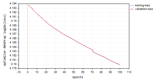
These optimizers are applied to the Stochastic Gradient Descent algorithm during backpropagation.

01: Root Mean Square Propagation(RMSProp)

This optimization algorithm aims to address the limitations of stochastic Gradient Descent (SGD) by adapting the learning rate for each weight and bias parameter based on their historical gradients.

Problem with SGD:

SGD updates weights and biases using the current gradient and a fixed learning rate. However, in complex functions like neural networks, the magnitude of gradients can vary significantly for different parameters. This can lead to slow convergence as parameters with small gradients might update very slowly, hindering overall learning also SGD can cause large oscillations as parameters with large gradients might experience excessive swings during updates, making the learning process unstable.

Theory:

Here's the core idea behind RMSprop:

Maintain an Exponential Moving Average (EMA) of squared gradients. For each parameter, RMSprop tracks an exponentially decaying average of the squared gradients. This average reflects the recent history of how much the parameter should be updated.
Normalize the Gradient. The current gradient for each parameter is divided by the square root of the EMA of squared gradients, along with a small smoothing term (usually denoted by ε) to avoid division by zero.
Update the Parameter. The normalized gradient is multiplied by the learning rate to determine the update for the parameter.

where:

EMA of squared gradients at time step t

Decay rate (hyperparameter, typically between 0.9 and 0.999) - controls the influence of past gradients

Gradient of the loss function with respect to parameter w at time step t

Parameter value at time step t

Updated parameter value at time step t+1

η: Learning rate (hyperparameter)

ε: Smoothing term (usually a small value like 1e-8)

class OptimizerRMSprop
  {
protected:
   double m_learning_rate;
   double m_decay_rate;
   double m_epsilon;
   
   matrix<double> cache;
   
   //Dividing double/matrix causes compilation error | this is the fix to the issue
   matrix divide(const double numerator, const matrix &denominator)
    {
      matrix res = denominator;
      
      for (ulong i=0; i<denominator.Rows(); i++)
        res.Row(numerator / denominator.Row(i), i);
     return res;
    }
    
public:
                     OptimizerRMSprop(double learning_rate=0.01, double decay_rate=0.9, double epsilon=1e-8);
                    ~OptimizerRMSprop(void);
                    
                    virtual void update(matrix& parameters, matrix& gradients);
  };
//+------------------------------------------------------------------+
//|                                                                  |
//+------------------------------------------------------------------+
OptimizerRMSprop::OptimizerRMSprop(double learning_rate=0.01, double decay_rate=0.9, double epsilon=1e-8):
 m_learning_rate(learning_rate),
 m_decay_rate(decay_rate),
 m_epsilon(epsilon)
 {
 
 }
//+------------------------------------------------------------------+
//|                                                                  |
//+------------------------------------------------------------------+
OptimizerRMSprop::~OptimizerRMSprop(void)
 {
 
 }
//+------------------------------------------------------------------+
//|                                                                  |
//+------------------------------------------------------------------+
void OptimizerRMSprop::update(matrix &parameters,matrix &gradients)
 {
 
   if (cache.Rows()!=parameters.Rows() || cache.Cols()!=parameters.Cols())
    {
     cache.Init(parameters.Rows(), parameters.Cols());
     cache.Fill(0.0);
    }
     
//---
    
    cache += m_decay_rate * cache + (1 - m_decay_rate) * MathPow(gradients, 2);
    parameters -= divide(m_learning_rate, cache + m_epsilon) * gradients;
 }

Going with 100 epochs and 0.0001, same default values used for the previous optimizers. The neural network failed to converge for 100 epochs as it provided approximately -319 and -324 accuracy in training and validation samples respectively. It seems it might need more than 1000 epochs at its pace assuming we don't overshoot the local minima for that large number of epochs.

HK      0       15:10:15.632    Optimization Algorithms testScript (EURUSD,H1)  --> Epoch [90/100] training -> loss 15164.85487215 accuracy -320.064 validation -> loss 15164.99272 accuracy -325.349 | Elapsed 0.031 Seconds 
HQ      0       15:10:15.663    Optimization Algorithms testScript (EURUSD,H1)  --> Epoch [91/100] training -> loss 15161.78717397 accuracy -319.999 validation -> loss 15161.92323 accuracy -325.283 | Elapsed 0.031 Seconds 
DO      0       15:10:15.694    Optimization Algorithms testScript (EURUSD,H1)  --> Epoch [92/100] training -> loss 15158.07142844 accuracy -319.921 validation -> loss 15158.20512 accuracy -325.203 | Elapsed 0.031 Seconds 
GE      0       15:10:15.727    Optimization Algorithms testScript (EURUSD,H1)  --> Epoch [93/100] training -> loss 15154.92004326 accuracy -319.854 validation -> loss 15155.05184 accuracy -325.135 | Elapsed 0.032 Seconds 
GS      0       15:10:15.760    Optimization Algorithms testScript (EURUSD,H1)  --> Epoch [94/100] training -> loss 15151.84229952 accuracy -319.789 validation -> loss 15151.97226 accuracy -325.069 | Elapsed 0.031 Seconds 
DH      0       15:10:15.796    Optimization Algorithms testScript (EURUSD,H1)  --> Epoch [95/100] training -> loss 15148.77653633 accuracy -319.724 validation -> loss 15148.90466 accuracy -325.003 | Elapsed 0.031 Seconds 
MF      0       15:10:15.831    Optimization Algorithms testScript (EURUSD,H1)  --> Epoch [96/100] training -> loss 15145.56414236 accuracy -319.656 validation -> loss 15145.69033 accuracy -324.934 | Elapsed 0.047 Seconds 
IL      0       15:10:15.869    Optimization Algorithms testScript (EURUSD,H1)  --> Epoch [97/100] training -> loss 15141.85430749 accuracy -319.577 validation -> loss 15141.97859 accuracy -324.854 | Elapsed 0.031 Seconds 
KJ      0       15:10:15.906    Optimization Algorithms testScript (EURUSD,H1)  --> Epoch [98/100] training -> loss 15138.40751503 accuracy -319.504 validation -> loss 15138.52969 accuracy -324.780 | Elapsed 0.032 Seconds 
PP      0       15:10:15.942    Optimization Algorithms testScript (EURUSD,H1)  --> Epoch [99/100] training -> loss 15135.31136641 accuracy -319.439 validation -> loss 15135.43169 accuracy -324.713 | Elapsed 0.046 Seconds 
NM      0       15:10:15.975    Optimization Algorithms testScript (EURUSD,H1)  --> Epoch [100/100] training -> loss 15131.73032246 accuracy -319.363 validation -> loss 15131.84854 accuracy -324.636 | Elapsed 0.032 Seconds

Loss vs Epoch plot: 100 epochs, 0.0001 learning rate.

Where to use RMSProp?

Good for non-stationary objectives, sparse gradients, simpler than Adam.

02: Adagrad (Adaptive Gradient Algorithm)

Adagrad is an optimizer for neural networks that utilizes an adaptive learning rate similar to RMSprop. However, Adagrad and RMSprop have some key differences in their approach.

Mathematics behind:

It Accumulates Past Gradients. Adagrad keeps track of the sum of squared gradients for each parameter throughout the training process. This accumulated value reflects how much a parameter has been updated in the past.
```
cache += MathPow(gradients, 2);
```
Normalizes the Gradient. The current gradient for each parameter is divided by the square root of the accumulated sum of squared gradients, along with a small smoothing term (usually denoted by ε) to avoid division by zero.
Update the Parameter. The normalized gradient is multiplied by the learning rate to determine the update for the parameter.
```
parameters -= divide(this.m_learning_rate,  MathSqrt(cache + this.m_epsilon)) * gradients;
```

nn_learning_rate = 0.0001, epochs = 100

  nn.fit(x_train, y_train, new OptimizerAdaGrad(nn_learning_rate), nn_epochs, nn_batch_size, show_batch);

Loss vs Epoch plot:

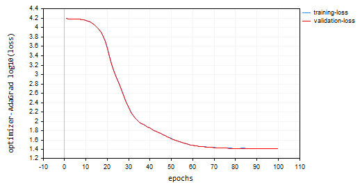
Adagrad had a steeper learning curve and it was very stable during the updates but it needed more than 100 epochs to converge as it ended up with approximate 44% accuracy both training and validation samples respectively.

RK      0       15:15:52.202    Optimization Algorithms testScript (EURUSD,H1)  --> Epoch [90/100] training -> loss 26.22261537 accuracy 0.445 validation -> loss 26.13118 accuracy 0.440 | Elapsed 0.031 Seconds 
ER      0       15:15:52.239    Optimization Algorithms testScript (EURUSD,H1)  --> Epoch [91/100] training -> loss 26.12443561 accuracy 0.447 validation -> loss 26.03635 accuracy 0.442 | Elapsed 0.047 Seconds 
NJ      0       15:15:52.277    Optimization Algorithms testScript (EURUSD,H1)  --> Epoch [92/100] training -> loss 26.11449352 accuracy 0.447 validation -> loss 26.02561 accuracy 0.442 | Elapsed 0.032 Seconds 
IQ      0       15:15:52.316    Optimization Algorithms testScript (EURUSD,H1)  --> Epoch [93/100] training -> loss 26.09263184 accuracy 0.448 validation -> loss 26.00461 accuracy 0.443 | Elapsed 0.046 Seconds 
NH      0       15:15:52.354    Optimization Algorithms testScript (EURUSD,H1)  --> Epoch [94/100] training -> loss 26.14277865 accuracy 0.447 validation -> loss 26.05529 accuracy 0.442 | Elapsed 0.032 Seconds 
HP      0       15:15:52.393    Optimization Algorithms testScript (EURUSD,H1)  --> Epoch [95/100] training -> loss 26.09559950 accuracy 0.448 validation -> loss 26.00845 accuracy 0.443 | Elapsed 0.047 Seconds 
PO      0       15:15:52.442    Optimization Algorithms testScript (EURUSD,H1)  --> Epoch [96/100] training -> loss 26.05409769 accuracy 0.448 validation -> loss 25.96754 accuracy 0.443 | Elapsed 0.046 Seconds 
PG      0       15:15:52.479    Optimization Algorithms testScript (EURUSD,H1)  --> Epoch [97/100] training -> loss 25.98822082 accuracy 0.450 validation -> loss 25.90384 accuracy 0.445 | Elapsed 0.032 Seconds 
PN      0       15:15:52.519    Optimization Algorithms testScript (EURUSD,H1)  --> Epoch [98/100] training -> loss 25.98781231 accuracy 0.450 validation -> loss 25.90438 accuracy 0.445 | Elapsed 0.047 Seconds 
EE      0       15:15:52.559    Optimization Algorithms testScript (EURUSD,H1)  --> Epoch [99/100] training -> loss 25.91146212 accuracy 0.451 validation -> loss 25.83083 accuracy 0.446 | Elapsed 0.031 Seconds 
CN      0       15:15:52.595    Optimization Algorithms testScript (EURUSD,H1)  --> Epoch [100/100] training -> loss 25.87412572 accuracy 0.452 validation -> loss 25.79453 accuracy 0.447 | Elapsed 0.047 Seconds

Advantages of Adagrad:

It converges faster for sparse features. In situations where many parameters have infrequent updates due to sparse features in the data, Adagrad can effectively reduce their learning rates, allowing faster convergence for those parameters.

Limitations of Adagrad:

Over time, the accumulated sum of squared gradients in Adagrad keeps growing, causing continuously decreasing learning rates for all parameters. This can eventually stall training progress.

When to Use Adagrad:

In sparse feature datasets: When dealing with datasets where many features have infrequent updates, Adagrad can be effective in speeding up convergence for those parameters.

During early stages of training: In some scenarios, the initial learning rate adjustments by Adagrad can be helpful before switching to another optimizer later in training.

03: Adaptive Moment Estimation(Adam)

A highly effective optimization algorithm widely used in training neural networks. It combines the strengths of AdaGrad and RMSprop to address their limitations and delivers efficient and stable learning.

Theory:

Adam has two key features;

Exponential Moving Average (EMA) of Gradients: Similar to RMSprop, Adam maintains an EMA of the squared gradients (cache) to capture the recent history of updates needed for each parameter.
Exponential Moving Average of Moments: Adam introduces another EMA (moment), which tracks the running average of the gradients themselves. This helps to mitigate the issue of vanishing gradients that can occur in some network architectures.

Normalization and Update:

Moment Update: The current gradient is utilized to update the EMA of moments (m_t).

this.moment = this.m_beta1 * this.moment + (1 -  this.m_beta1) * gradients;

Squared Gradient Update: The current squared gradient is used to update the EMA of squared gradients (cache_t).
```
this.cache = this.m_beta2 * this.cache + (1 -  this.m_beta2) * MathPow(gradients, 2);
```
Bias Correction: Both EMAs (moment_t and cache_t) are corrected for bias using exponential decay factors (β1 and β2) to ensure they are unbiased estimates of the true moments.
```
matrix moment_hat = this.moment / (1 - MathPow(this.m_beta1, this.time_step));
```
```
matrix cache_hat = this.cache / (1 - MathPow(this.m_beta2, this.time_step));
```
Normalization: Similar to RMSprop, the current gradient is normalized using the corrected EMAs and a small smoothing term (ε).
Parameter updates: The normalized gradient is multiplied by the learning rate (η) to determine the update for the parameter.
```
parameters -= (this.m_learning_rate * moment_hat) / (MathPow(cache_hat, 0.5) + this.m_epsilon);
```

This is how the constructor for Adam optimizer looks like:

OptimizerAdam(double learning_rate=0.01, double beta1=0.9, double beta2=0.999, double epsilon=1e-8);

I called it with the learning rate:

nn.fit(x_train, y_train, new OptimizerAdam(nn_learning_rate), nn_epochs, nn_batch_size, show_batch);

The resulting Loss vs Epoch plot:

adam loss vs epoch plot

Adam performed better than the prior optimizers apart from SGD, providing approximate 53% and 52% accuracy on training and validation training sample respectively.

MD      0       15:23:37.651    Optimization Algorithms testScript (EURUSD,H1)  --> Epoch [90/100] training -> loss 22.05051037 accuracy 0.533 validation -> loss 21.92528 accuracy 0.529 | Elapsed 0.047 Seconds 
DS      0       15:23:37.703    Optimization Algorithms testScript (EURUSD,H1)  --> Epoch [91/100] training -> loss 22.38393234 accuracy 0.526 validation -> loss 22.25178 accuracy 0.522 | Elapsed 0.046 Seconds 
OK      0       15:23:37.756    Optimization Algorithms testScript (EURUSD,H1)  --> Epoch [92/100] training -> loss 22.12091827 accuracy 0.532 validation -> loss 21.99456 accuracy 0.528 | Elapsed 0.063 Seconds 
OR      0       15:23:37.808    Optimization Algorithms testScript (EURUSD,H1)  --> Epoch [93/100] training -> loss 21.94438889 accuracy 0.535 validation -> loss 21.81944 accuracy 0.532 | Elapsed 0.047 Seconds 
NI      0       15:23:37.862    Optimization Algorithms testScript (EURUSD,H1)  --> Epoch [94/100] training -> loss 22.41965082 accuracy 0.525 validation -> loss 22.28371 accuracy 0.522 | Elapsed 0.062 Seconds 
LQ      0       15:23:37.915    Optimization Algorithms testScript (EURUSD,H1)  --> Epoch [95/100] training -> loss 22.27254037 accuracy 0.528 validation -> loss 22.13931 accuracy 0.525 | Elapsed 0.047 Seconds 
FH      0       15:23:37.969    Optimization Algorithms testScript (EURUSD,H1)  --> Epoch [96/100] training -> loss 21.93193893 accuracy 0.536 validation -> loss 21.80427 accuracy 0.532 | Elapsed 0.047 Seconds 
LG      0       15:23:38.024    Optimization Algorithms testScript (EURUSD,H1)  --> Epoch [97/100] training -> loss 22.41523220 accuracy 0.525 validation -> loss 22.27900 accuracy 0.522 | Elapsed 0.063 Seconds 
MO      0       15:23:38.077    Optimization Algorithms testScript (EURUSD,H1)  --> Epoch [98/100] training -> loss 22.23551304 accuracy 0.529 validation -> loss 22.10466 accuracy 0.526 | Elapsed 0.046 Seconds 
QF      0       15:23:38.129    Optimization Algorithms testScript (EURUSD,H1)  --> Epoch [99/100] training -> loss 21.96662717 accuracy 0.535 validation -> loss 21.84087 accuracy 0.531 | Elapsed 0.063 Seconds 
GM      0       15:23:38.191    Optimization Algorithms testScript (EURUSD,H1)  --> Epoch [100/100] training -> loss 22.29715377 accuracy 0.528 validation -> loss 22.16686 accuracy 0.524 | Elapsed 0.062 Seconds

Advantages of Adam:

It converges faster: Adam often converges faster than SGD and can be more efficient than RMSprop in various scenarios.
Less Sensitive to Learning Rate: Compared to SGD, Adam is less sensitive to the choice of learning rate, making it more robust.
Suitable for Non-Convex Loss Functions: It can effectively handle non-convex loss functions common in deep learning tasks.
Wide Applicability: Adam's combination of features makes it a widely applicable optimizer for various network architectures and datasets.

Disadvantages:

Hyperparameter Tuning: While generally less sensitive, Adam still requires tuning of hyperparameters like learning rate and decay rates for optimal performance.
Memory Usage: Maintaining the EMAs can lead to slightly higher memory consumption compared to SGD.

Where to use Adam?

Use Adam (Adaptive Moment Estimation) for your neural network training when you want:

Faster convergence. You want your network to be less sensitive to the learning rate and, when you want adaptive learning rate with momentum.

04: Adadelta(Adaptive Learning with delta)

This is another optimization algorithm used in neural networks, it shares some similarities with SGD and RMSProp offering an adaptive learning rate with a specific momentum term.

Adadelta aims to address SGD fixed learning rate which leads to slow convergence and oscillations. It employs an adaptive learning rate that adjusts based on past squared gradients, similar to RMSProp.

Maths behind:

Maintain an Exponential Moving Average (EMA) of squared deltas, Adadelta calculates an EMA of the squared differences between consecutive parameter updates (deltas) for each parameter. This reflects the recent history of how much the parameter has changed.
```
this.cache = m_decay_rate * this.cache + (1 - m_decay_rate) * MathPow(gradients, 2);
```
Adaptive Learning Rate: The current squared gradient for a parameter is divided by the EMA of squared deltas (with a smoothing term). This effectively serves as an adaptive learning rate, controlling the update size for each parameter.
```
matrix delta = lr * sqrt(this.cache + m_epsilon) / sqrt(pow(gradients, 2) + m_epsilon);
```
Momentum: Adadelta incorporates a momentum term that considers the previous update for the parameter, similar to momentum SGD. This helps to accumulate gradients and potentially escape local minima.
```
matrix momentum_term = this.m_gamma * parameters + (1 - this.m_gamma) * gradients;

parameters -= delta * momentum_term;
```

Where:

: EMA of squared deltas at time step t

: Decay rate (hyperparameter, typically between 0.9 and 0.999)

: Gradient of the loss function with respect to parameter w at time step t

: Parameter value at time step t

: Updated parameter value at time step t+1

ε: Smoothing term (usually a small value like 1e-8)

γ: Momentum coefficient (hyperparameter, typically between 0 and 1)

Adavantages of Adadelta:

Converges Faster: Compared to SGD with a fixed learning rate, Adadelta can often converge faster, especially for problems with non-stationary gradients.
It uses Momentum for Escaping Local Minima: The momentum term helps to accumulate gradients and potentially escape local minima in the loss function.
Less Sensitive to Learning Rate: Similar to RMSprop, Adadelta is less sensitive to the specific learning rate chosen than SGD.

Disadvantages of Adadelta:

Requires tuning of hyperparameters like the decay rate (ρ) and momentum coefficient (γ) for optimal performance.

OptimizerAdaDelta(double learning_rate=0.01, double decay_rate=0.95, double gamma=0.9, double epsilon=1e-8);

Computationally expensive: Maintaining the EMA and incorporating momentum slightly increases computational cost compared to SGD.

Where to use Adadelta:

Adadelta can be a valuable alternative in certain scenarios:

Non-stationary gradients. If your problem exhibits non-stationary gradients, Adadelta's adaptive learning rate with momentum might be beneficial.
In situations where escaping local minima is crucial, Adadelta's momentum term might be advantageous.

I trained the model using adadelta, for 100 epochs, 0.0001 learning rate. Everything was the same as used in other optimizers:

nn.fit(x_train, y_train, new OptimizerAdaDelta(nn_learning_rate), nn_epochs, nn_batch_size, show_batch);

Loss vs epoch plot:

adadelta loss vs epochs plot

The Adadelta optimizer failed to learn anything as it provided the same loss value of 15625 and an accuracy of approximately -335 on training and validation samples, It looks like what was done with RMSProp.

NP      0       15:32:30.664    Optimization Algorithms testScript (EURUSD,H1)  --> Epoch [90/100] training -> loss 15625.71263806 accuracy -329.821 validation -> loss 15626.09899 accuracy -335.267 | Elapsed 0.062 Seconds 
ON      0       15:32:30.724    Optimization Algorithms testScript (EURUSD,H1)  --> Epoch [91/100] training -> loss 15625.71263806 accuracy -329.821 validation -> loss 15626.09899 accuracy -335.267 | Elapsed 0.063 Seconds 
IK      0       15:32:30.788    Optimization Algorithms testScript (EURUSD,H1)  --> Epoch [92/100] training -> loss 15625.71263806 accuracy -329.821 validation -> loss 15626.09899 accuracy -335.267 | Elapsed 0.062 Seconds 
JQ      0       15:32:30.848    Optimization Algorithms testScript (EURUSD,H1)  --> Epoch [93/100] training -> loss 15625.71263806 accuracy -329.821 validation -> loss 15626.09899 accuracy -335.267 | Elapsed 0.063 Seconds 
RO      0       15:32:30.914    Optimization Algorithms testScript (EURUSD,H1)  --> Epoch [94/100] training -> loss 15625.71263806 accuracy -329.821 validation -> loss 15626.09899 accuracy -335.267 | Elapsed 0.062 Seconds 
PE      0       15:32:30.972    Optimization Algorithms testScript (EURUSD,H1)  --> Epoch [95/100] training -> loss 15625.71263806 accuracy -329.821 validation -> loss 15626.09899 accuracy -335.267 | Elapsed 0.063 Seconds 
CS      0       15:32:31.029    Optimization Algorithms testScript (EURUSD,H1)  --> Epoch [96/100] training -> loss 15625.71263806 accuracy -329.821 validation -> loss 15626.09899 accuracy -335.267 | Elapsed 0.047 Seconds 
DI      0       15:32:31.086    Optimization Algorithms testScript (EURUSD,H1)  --> Epoch [97/100] training -> loss 15625.71263806 accuracy -329.821 validation -> loss 15626.09899 accuracy -335.267 | Elapsed 0.062 Seconds 
DG      0       15:32:31.143    Optimization Algorithms testScript (EURUSD,H1)  --> Epoch [98/100] training -> loss 15625.71263806 accuracy -329.821 validation -> loss 15626.09899 accuracy -335.267 | Elapsed 0.063 Seconds 
FM      0       15:32:31.202    Optimization Algorithms testScript (EURUSD,H1)  --> Epoch [99/100] training -> loss 15625.71263806 accuracy -329.821 validation -> loss 15626.09899 accuracy -335.267 | Elapsed 0.046 Seconds 
GI      0       15:32:31.258    Optimization Algorithms testScript (EURUSD,H1)  --> Epoch [100/100] training -> loss 15625.71263806 accuracy -329.821 validation -> loss 15626.09899 accuracy -335.267 | Elapsed 0.063 Seconds

05: Nadam: Nesterov-accelerated Adaptive Moment Estimation

This optimization algorithm combines the strengths of two popular optimizers: Adam (Adaptive Moment Estimation) and Nesterov Momentum. It aims to achieve faster convergence and potentially better performance compared to Adam, especially in situations with noisy gradients.

Nadam's Approach:

It inherits the core functionalities of Adam:

class OptimizerNadam: protected OptimizerAdam
  {
protected:
   double m_gamma;
   
    
public:
                     OptimizerNadam(double learning_rate=0.01, double beta1=0.9, double beta2=0.999, double gamma=0.9, double epsilon=1e-8);
                    ~OptimizerNadam(void);
                    
                    virtual void update(matrix &parameters, matrix &gradients);
  };
//+------------------------------------------------------------------+
//|  Initializes the Adam optimizer with hyperparameters.            |   
//|                                                                  |
//|  learning_rate: Step size for parameter updates                  |
//|  beta1: Decay rate for the first moment estimate                 |
//|     (moving average of gradients).                               |
//|  beta2: Decay rate for the second moment estimate                |
//|     (moving average of squared gradients).                       |
//|  epsilon: Small value for numerical stability.                   |
//+------------------------------------------------------------------+
OptimizerNadam::OptimizerNadam(double learning_rate=0.010000, double beta1=0.9, double beta2=0.999, double gamma=0.9, double epsilon=1e-8)
:OptimizerAdam(learning_rate, beta1, beta2, epsilon),
 m_gamma(gamma)
 {
 
 }

Including:

Maintaining EMAs (Exponential Moving Averages): It tracks the EMA of squared gradients (cache_t) and the EMA of moments (m_t), similar to Adam.
Adaptive learning rate Calculations: Based on these EMAs, it calculates an adaptive learning rate that adjusts for each parameter.
It incorporates Nesterov Momentum: Nadam borrows the concept of Nesterov Momentum from SGD with Nesterov Momentum. This involves:
"Peek" Gradient: Before updating the parameter based on the current gradient, Nadam estimates a "peek" gradient using the current gradient and the momentum term.
Update with "Peek" Gradient: The parameter update is then performed using this "peek" gradient, potentially leading to faster convergence and improved handling of noisy gradients.

Maths behind Nadam:

Updating EMA of moments (same as Adam)
Updating EMA of squared gradients (same as Adam)
Bias correction for moments (same as Adam)
Bias correction for squared gradients (same as Adam)
Nesterov momentum (using previous gradient estimate)
Update previous gradient estimate

Update parameter with Nesterov momentum

matrix nesterov_moment = m_gamma * moment_hat + (1 - m_gamma) * gradients; // Nesterov accelerated gradient

parameters -= m_learning_rate * nesterov_moment / sqrt(cache_hat + m_epsilon); // Update parameters

Advantages of Nadam:

It is faster: Compared to Adam, Nadam can potentially achieve faster convergence, especially for problems with noisy gradients.
It is better at handling noisy gradients: The Nesterov momentum term in Nadam can help to smooth out noisy gradients and lead to better performance.
It has Adam's advantages: It retains the benefits of Adam, such as adaptivity and less sensitivity to learning rate selection.

Disadvantages:

Requires tuning of hyperparameters like learning rate, decay rates, and momentum coefficient for optimal performance.
While Nadam shows promise, it may not always outperform Adam in all scenarios. Further research and experimentation are needed.

Where to Use Nadam?

Can be a great alternative to Adam in problems where there are noisy gradients.

I called Nadam with default parameters and the same learning rate we used for all prior discussed optimizers. I ended up second best from Adam providing approximately 47% accuracy on both training and validation sets. Nadam made a lot of oscillations around the local minima than other discussed methods in this article.

IL      0       15:37:56.549    Optimization Algorithms testScript (EURUSD,H1)  --> Epoch [90/100] training -> loss 25.23632476 accuracy 0.466 validation -> loss 25.06902 accuracy 0.462 | Elapsed 0.062 Seconds 
LK      0       15:37:56.619    Optimization Algorithms testScript (EURUSD,H1)  --> Epoch [91/100] training -> loss 24.60851222 accuracy 0.479 validation -> loss 24.44829 accuracy 0.475 | Elapsed 0.078 Seconds 
RS      0       15:37:56.690    Optimization Algorithms testScript (EURUSD,H1)  --> Epoch [92/100] training -> loss 24.68657614 accuracy 0.477 validation -> loss 24.53442 accuracy 0.473 | Elapsed 0.078 Seconds 
IJ      0       15:37:56.761    Optimization Algorithms testScript (EURUSD,H1)  --> Epoch [93/100] training -> loss 24.89495551 accuracy 0.473 validation -> loss 24.73423 accuracy 0.469 | Elapsed 0.063 Seconds 
GQ      0       15:37:56.832    Optimization Algorithms testScript (EURUSD,H1)  --> Epoch [94/100] training -> loss 25.25899364 accuracy 0.465 validation -> loss 25.09940 accuracy 0.461 | Elapsed 0.078 Seconds 
QI      0       15:37:56.901    Optimization Algorithms testScript (EURUSD,H1)  --> Epoch [95/100] training -> loss 25.17698272 accuracy 0.467 validation -> loss 25.01065 accuracy 0.463 | Elapsed 0.063 Seconds 
FP      0       15:37:56.976    Optimization Algorithms testScript (EURUSD,H1)  --> Epoch [96/100] training -> loss 25.36663261 accuracy 0.463 validation -> loss 25.20273 accuracy 0.459 | Elapsed 0.078 Seconds 
FO      0       15:37:57.056    Optimization Algorithms testScript (EURUSD,H1)  --> Epoch [97/100] training -> loss 23.34069092 accuracy 0.506 validation -> loss 23.19590 accuracy 0.502 | Elapsed 0.078 Seconds 
OG      0       15:37:57.128    Optimization Algorithms testScript (EURUSD,H1)  --> Epoch [98/100] training -> loss 23.48894694 accuracy 0.503 validation -> loss 23.33753 accuracy 0.499 | Elapsed 0.078 Seconds 
ON      0       15:37:57.203    Optimization Algorithms testScript (EURUSD,H1)  --> Epoch [99/100] training -> loss 23.03205165 accuracy 0.512 validation -> loss 22.88233 accuracy 0.509 | Elapsed 0.062 Seconds 
ME      0       15:37:57.275    Optimization Algorithms testScript (EURUSD,H1)  --> Epoch [100/100] training -> loss 24.98193438 accuracy 0.471 validation -> loss 24.82652 accuracy 0.467 | Elapsed 0.079 Seconds

Below was the loss vs epoch graph:

nadam loss vs epoch graph

Final Thoughts

The best optimizer choice depends on your specific problem, dataset, network architecture and, parameters . Experimentation is key to finding the most effective optimizer for your neural network training task. Adam proves to be the best optimizer for many neural network due to its ability to converge faster, it is less sensitive to learning rate and adapts its learning rate with momentum. It is a good choice to try first, especially for complex problem or when you are not sure which optimizer to use initially.

Best wishes.

Track development of machine learning models and much more discussed in this article series on this GitHub repo.

Attachments:

File	Description/Usage
MatrixExtend.mqh	Has additional functions for matrix manipulations.
metrics.mqh	Contains functions and code to measure the performance of ML models.
preprocessing.mqh	The library for pre-processing raw input data to make it suitable for Machine learning models usage.
plots.mqh	Library for plotting vectors and matrices
optimizers.mqh	An Include file containing all neural network optimizers discussed in this article
cross_validation.mqh	A library containing cross validation Techniques
Tensors.mqh	A library containing Tensors, algebraic 3D matrices objects programmed in plain-MQL5 language
Regressor Nets.mqh	Contains neural networks for solving a regression problem
Optimization Algorithms testScript.mq5	A script for running the code from all the include files and the dataset/This is the main file
airfoil_noise_data.csv	Airfoil regression problem data

Attached files |

Download ZIP

Code_k_Files.zip (39.41 KB)

Warning: All rights to these materials are reserved by MetaQuotes Ltd. Copying or reprinting of these materials in whole or in part is prohibited.

Introduction

What are the Neural Network Optimizers?

01: Stochastic Gradient Descent Algorithm(SGD)

02: Batch Gradient Descent Algorithm(BGD):

03: Mini-Batch Gradient Descent:

Types of Neural Network Optimizers

01: Root Mean Square Propagation(RMSProp)

02: Adagrad (Adaptive Gradient Algorithm)

03: Adaptive Moment Estimation(Adam)

04: Adadelta(Adaptive Learning with delta)

05: Nadam: Nesterov-accelerated Adaptive Moment Estimation

Final Thoughts

Other articles by this author