Comet Tail Algorithm (CTA)
Contents
1. Introduction
2. Algorithm implementation
3.Test results
1. Introduction
In the world of astronomy, comets have always been of particular interest to scientists and researchers. These unique space objects, consisting mainly of ice, dust and gases, are an important source of information about the processes occurring in outer space. One of the most noticeable and impressive aspects of comets is their tail, which forms as the comet approaches the Sun.
The Sun plays a key role in the formation of a comet's tail. Its radiation and solar wind cause the evaporation and destruction of material on the comet's surface. This process leads to the formation of a comet tail — an area of dust, gases, and ionized particles that are pushed away from the comet by the solar wind and the Sun's gravity.
In this article, we will look at the CTA (Comet Tail Algorithm) optimization algorithm inspired by this unique astronomical phenomenon. The CTA algorithm uses the concept of comet motion and its tails to find optimal solutions to optimization problems. We will take a detailed look at the movement of the comet and its tail, as well as the role of the Sun in these processes. We will also discuss how these concepts are applied in the CTA algorithm to effectively find optimal solutions.
Comets are small bodies in the solar system that evaporate and release gases as they approach the Sun. This process is called sublimation. Comets typically have highly elliptical orbits, as well as a wide range of orbital periods - from a few years to potentially several million years.
The movement of a comet and its tail is closely related to the influence of the Sun. The heat of the Sun causes the comet ice to turn into gases, causing the coma (the shell of gases surrounding the comet nucleus) to expand. Pressure from solar radiation and high-speed solar particles (solar wind) can blow coma dust and gas away from the Sun, sometimes forming a long, bright tail. In addition, solar radiation and solar wind cause ionization of gases in the comet's tail, causing it to glow.
In the context of the CTA algorithm, we can think of each solution as comet tail particles moving in the solution space. The comet nucleus represents the best solution, and the particles in the tail are derivatives of the solution emanating from the nucleus. This representation allows the algorithm to "learn" the solution space and adapt to its features.
2. Algorithm implementation
Let's take a closer look at the motion of the comet and its tail, which are key elements in this algorithm, as well as the role of the Sun in these processes.
Comet movement:
- The comet moves in an elliptical orbit around the Sun.
- As a comet approaches the Sun, it begins to emit gas and dust, forming a cometary tail.
- The comet's motion is determined by the gravitational attraction of the Sun, as well as repulsion from the solar wind and solar radiation.
- The comet moves along its orbit, and its tail is always directed in the direction opposite to the Sun.
Comet tail motion:
- The comet's gas tail consists of ionized gases that are "thrown out" from the comet's nucleus by the solar wind.
- Solar wind is a stream of charged particles emanating from the Sun. It "blows away" the comet's gas tail, directing it opposite to the Sun.
- The dust tail of a comet consists of larger particles that are "thrown out" from the comet's nucleus by solar radiation.
- Solar radiation exerts pressure on the dust particles, slightly deflecting them from the direction of the comet's motion, forming a curved dust tail.
Role of the Sun:
- The Sun is the central object around which the comet moves in its orbit.
- The gravitational attraction of the Sun determines the comet's motion along an elliptical orbit.
- The solar wind and solar radiation "shape" the comet's tail, directing it opposite to the Sun.
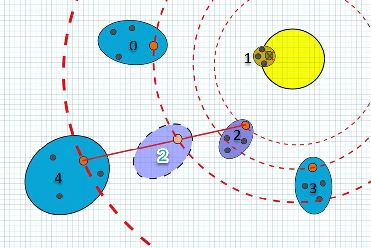
Figure 1. Comet shape and size in the context of the CTA algorithm as a function of distance to the star (best global solution)
Comet number 1 came too close to the sun and evaporated. However, in the algorithm, the destruction of the comet does not actually occur. Instead, the formation of a tail cloud with a center corresponding to the center of the star continues. This means that the smaller the tail cloud, the more intensively the refinement of the solution in the region of the comet occurs. Conversely, the larger the tail size, the more intensively the search space is explored. In this case, the axes of the ellipses of all comets are always directed away from the star, that is, away from the current best global solution.
The logic of the algorithm allows us to regulate the expansion coefficients of comet clouds both in the direction of expansion with distance from the star, and in the direction of decrease. It is also possible to adjust the degree of flattening of the ellipses depending on the radius of the comet's orbit. We can even direct the comet's tail not away from the star, but towards the star (if desired).
Figure 1 also shows the moment of the conditional migration of comet number 2 to a new orbit (circled number 2). This occurs during the exchange of matter between the nuclei of two comets. In the figure, comet 2 borrows matter from comet 4. If a better solution is found in the process of exchange of matter between comets, then the corresponding comet (whose matter was forming at that moment) moves to a new orbit.
The size of the comet's tail and its displacement relative to the nucleus depending on the distance to the star can be conditionally calculated according to a linear law. In this case, the maximum distance equal to 1 corresponds to the range of minimum and maximum values for the corresponding optimized coordinate of the problem. This approach allows us to describe the change in the parameters of a comet's tail depending on the distance to the star in a simple and clear way.
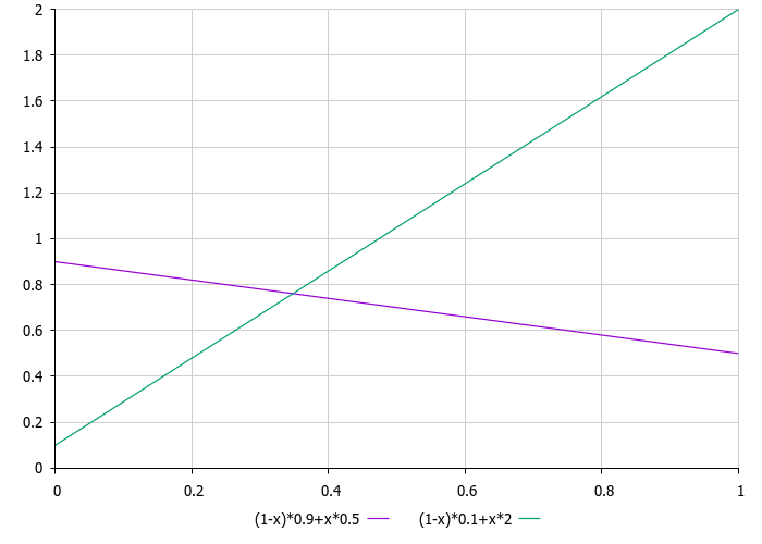
Figure 2. Graphs of the dependence of the comet's trail displacement ratios (purple) and the trail size (green) depending on the distance to the star
So, we have developed the laws of change of shape and size of the particle cloud for comets, so we can summarize the conclusions about the possible properties of the algorithm. The main properties of the algorithm inspired by the comet trail, taking into account the direction of the tail from the Sun (global optimum) and the search both on the best and less optimal solutions, can be as follows:
1. Evaporation and evolution of solutions. The algorithm can use a process of evaporation and evolution of solutions, in which both the best and less optimal solution regions can be explored.
2. Multivariance. The algorithm may strive to generate a variety of solution options that reflect different levels of optimality, similar to the diversity of composition in a comet tail.
3. Adaptability to external factors. As the comet responds to solar irradiation, the algorithm can be adaptive to changes in the environment or the objective function.
4. Search for global optimum. The direction of the tail away from the Sun may symbolize the algorithm's desire to find a global optimum, while at the same time taking into account less optimal solutions in order to avoid premature convergence to local optima.
Let's write a sketch of the algorithm in pseudocode:
1. Generate comet nuclei randomly.
2. From comet nuclei create their tails - particles with a normal distribution with the nucleus in the center.
3. Calculate the fitness of comet particles.
4. Update global solution.
5. Assign the best particle of the corresponding comet as its nucleus.
6. For each coordinate of the comet particles, do the following:
With the probability of 0.6, either:
Create particles with a normal distribution with a comet nucleus at the center.
Or:
Create a comet particle using the coordinates of the nuclei of two randomly selected comets.
7. Update global solution.
8. Assign the best particle of the corresponding comet as its nucleus.
9. Repeat from p. 6 until the stop criterion is met.
There is no need to write a specific structure for the CTA algorithm. The basic structure of the agent, used to exchange decisions between the algorithm and the executing program, is sufficient to describe comets and their particles. Let's remember what this structure looks like.
The S_AO_Agent structure contains two fields:
- c[] - the array stores the agent coordinates in the solution space.
- f - agent fitness used to evaluate the solution quality.
In the context of the CTA algorithm, we will use this structure to describe both the comets themselves and the particles of their tails.
//——————————————————————————————————————————————————————————————————————————————
struct S_AO_Agent
{
    double c []; //coordinates
    double f;    //fitness
};
//——————————————————————————————————————————————————————————————————————————————
Let's define the C_AO_CTA class, which is an inheritor of the C_AO class.
- C_AO_CTA () - the constructor initializes the class object with predefined values. It also sets some parameters of the algorithm, such as the population size (popSize), number of comets (cometsNumb), tail length coefficient (tailLengthKo), maximum and minimum shift coefficients (maxShiftCoef and minShiftCoef), as well as the maximum and minimum size coefficients (maxSizeCoef and minSizeCoef).
- SetParams() sets the algorithm parameters based on the values in the params array.
- Init() initializes the algorithm with the specified search ranges and number of epochs.
- The Moving() and Revision() methods implement the main logic of the algorithm.
The comets[] field is an array of S_AO_Agent type objects, which represents comets in the algorithm.
The tailLength[], maxSpaceDistance[] and partNumber private fields are used for the internal operation of the algorithm.
//——————————————————————————————————————————————————————————————————————————————
class C_AO_CTA : public C_AO
{
  public: //--------------------------------------------------------------------
  ~C_AO_CTA () { }

  C_AO_CTA ()
  {
    ao_name = "CTA";
    ao_desc = "Comet Tail Algorithm";
    ao_link = "https://www.mql5.com/ru/articles/14841";

    popSize      = 50;   //population size
    cometsNumb   = 5;    //number of comets
    tailLengthKo = 0.2;  //tail length coefficient
    maxShiftCoef = 0.9;
    minShiftCoef = 0.5;
    maxSizeCoef  = 0.1;
    minSizeCoef  = 1.5;

    ArrayResize (params, 7);

    params [0].name = "popSize";       params [0].val = popSize;
    params [1].name = "cometsNumb";    params [1].val = cometsNumb;
    params [2].name = "tailLengthKo";  params [2].val = tailLengthKo;
    params [3].name = "maxShiftCoef";  params [3].val = maxShiftCoef;
    params [4].name = "minShiftCoef";  params [4].val = minShiftCoef;
    params [5].name = "maxSizeCoef";   params [5].val = maxSizeCoef;
    params [6].name = "minSizeCoef";   params [6].val = minSizeCoef;
  }

  void SetParams ()
  {
    popSize      = (int)params [0].val;
    cometsNumb   = (int)params [1].val;
    tailLengthKo = params      [2].val;
    maxShiftCoef = params      [3].val;
    minShiftCoef = params      [4].val;
    maxSizeCoef  = params      [5].val;
    minSizeCoef  = params      [6].val;
  }

  bool Init (const double &rangeMinP  [], //minimum search range
             const double &rangeMaxP  [], //maximum search range
             const double &rangeStepP [], //step search
             const int     epochsP = 0);  //number of epochs

  void Moving   ();
  void Revision ();
  void Injection (const int popPos, const int coordPos, const double value);

  //----------------------------------------------------------------------------
  int    cometsNumb;    //number of comets
  double tailLengthKo;  //tail length coefficient
  double maxShiftCoef;  //maximum shift coefficient
  double minShiftCoef;  //minimum shift coefficient
  double maxSizeCoef;   //maximum size coefficient
  double minSizeCoef;   //minimum size coefficient

  S_AO_Agent comets [];

  private: //-------------------------------------------------------------------
  int    epochs;
  int    epochNow;
  double tailLength       [];
  double maxSpaceDistance []; //maximum distance in space
  int    partNumber; //number of particles
};
//——————————————————————————————————————————————————————————————————————————————
Define the Init method in the C_AO_CTA class. This method initializes the algorithm with the given search ranges and number of epochs. Description of each step:
1. if (!StandardInit (rangeMinP, rangeMaxP, rangeStepP)) return false; - the code calls the StandardInit method with the specified search ranges. If StandardInit returns 'false', the Init method also immediately returns 'false'.
2. ArrayResize (comets, cometsNumb); - resize the comets array size according to the number of comets.
3. Coordinates and fitness function value are initialized for each comet inside the "for" loop.
4. ArrayResize (tailLength, coords); ArrayResize (maxSpaceDistance, coords); - change the size of the tailLength and maxSpaceDistance arrays according to the number of coordinates.
5. Inside the following "for" loop, the maximum distance in space and the tail length are calculated for each coordinate.
6. partNumber = popSize / cometsNumb; - calculate the number of particles in the tail of each comet.
//——————————————————————————————————————————————————————————————————————————————
bool C_AO_CTA::Init (const double &rangeMinP [], //minimum search range
                     const double &rangeMaxP  [], //maximum search range
                     const double &rangeStepP [], //step search
                     const int     epochsP = 0)   //number of epochs
{
  if (!StandardInit (rangeMinP, rangeMaxP, rangeStepP)) return false;

  //----------------------------------------------------------------------------
  epochs   = epochsP;
  epochNow = 0;

  ArrayResize (comets, cometsNumb);
  for (int i = 0; i < cometsNumb; i++)
  {
    ArrayResize (comets [i].c, coords);
    comets [i].f = -DBL_MAX;
  }

  ArrayResize (tailLength,       coords);
  ArrayResize (maxSpaceDistance, coords);

  for (int i = 0; i < coords; i++)
  {
    maxSpaceDistance [i] = rangeMax [i] - rangeMin [i];
    tailLength       [i] = maxSpaceDistance [i] * tailLengthKo;
  }

  partNumber = popSize / cometsNumb;

  return true;
}
//——————————————————————————————————————————————————————————————————————————————
The formation of particles in comet tails occurs in the Moving() method of the C_AO_CTA class. The main steps of the method:
1. The function starts by incrementing the epochNow epoch counter and initializing the cnt, min and max local variables.
2. If revision is 'false', then the comet coordinates are initialized within the specified rangeMin and rangeMax ranges. Particles (agents) are then created around each comet using the Gaussian distribution within the range determined by tailLength.
3. If revision is 'true', then the position of particles (agents) is updated. The coefTail and coefSize coefficients are calculated for each particle. They define the displacement and size of the comet's tail depending on the distance to the cB central point. These coefficients are used to determine the new position of the particle within a range limited by the tail length.
4. If the u.RNDprobab() probability is less than 0.6, then the new position of the particle is calculated using the Gaussian distribution. Otherwise, the new position of the particle is calculated as a linear combination of the coordinates of the nuclei of two other randomly selected comets.
5. In all cases, the new coordinates of the particle are limited to the rangeMin and rangeMax and are discretized with the step of rangeStep.
The general idea of this method is to model the motion and behavior of comets in a CTA algorithm, where particles (agents) represent the comet's tail, and their coordinates and tail size depend on the distance to the global best solution (the Sun).
//——————————————————————————————————————————————————————————————————————————————
void C_AO_CTA::Moving ()
{
  epochNow++;
  int    cnt = 0;
  double min = 0.0;
  double max = 0.0;

  //----------------------------------------------------------------------------
  if (!revision)
  {
    for (int i = 0; i < cometsNumb; i++)
    {
      for (int c = 0; c < coords; c++)
      {
        comets [i].c [c] = u.RNDfromCI (rangeMin [c], rangeMax [c]);
        comets [i].c [c] = u.SeInDiSp  (comets [i].c [c], rangeMin [c], rangeMax [c], rangeStep [c]);
      }
    }

    for (int i = 0; i < cometsNumb; i++)
    {
      for (int p = 0; p < partNumber; p++)
      {
        for (int c = 0; c < coords; c++)
        {
          min = comets [i].c [c] - tailLength [c] * 0.5; if (min < rangeMin [c]) min = rangeMin [c];
          max = comets [i].c [c] + tailLength [c] * 0.5; if (max > rangeMax [c]) max = rangeMax [c];

          a [cnt].c [c] = u.GaussDistribution (comets [i].c [c], min, max, 1);
          a [cnt].c [c] = u.SeInDiSp  (a [cnt].c [c], rangeMin [c], rangeMax [c], rangeStep [c]);
        }

        cnt++;
      }
    }

    revision = true;
    return;
  }

  //----------------------------------------------------------------------------
  cnt             = 0;
  double coefTail = 0.0;
  double coefSize = 0.0;

  for (int i = 0; i < cometsNumb; i++)
  {
    for (int p = 0; p < partNumber; p++)
    {
      for (int c = 0; c < coords; c++)
      {
        if (u.RNDprobab () < 0.6)
        {
          coefTail = fabs (comets [i].c [c] - cB [c]) / maxSpaceDistance [c];
          coefSize = coefTail;

          //(1-x)*0.9+x*0.5
          coefTail = (1 - coefTail) * maxShiftCoef + coefTail * minShiftCoef;

          //(1-x)*0.1+x*0.9
          coefSize = (1 - coefSize) * maxSizeCoef + coefSize * minSizeCoef;

          if (cB [c] * Dir > comets [i].c [c] * Dir)
          {
            min = comets [i].c [c] - tailLength [c] * coefTail         * coefSize;
            max = comets [i].c [c] + tailLength [c] * (1.0 - coefTail) * coefSize;
          }
          if (cB [c] * Dir < comets [i].c [c] * Dir)
          {
            min = comets [i].c [c] - tailLength [c] * (1.0 - coefTail) * coefSize;
            max = comets [i].c [c] + tailLength [c] * (coefTail)*coefSize;
          }
          if (cB [c] == comets [i].c [c])
          {
            min = comets [i].c [c] - tailLength [c] * 0.1;
            max = comets [i].c [c] + tailLength [c] * 0.1;
          }

          if (min < rangeMin [c]) min = rangeMin [c];
          if (max > rangeMax [c]) max = rangeMax [c];

          a [cnt].c [c] = u.GaussDistribution (comets [i].c [c], min, max, Power);
          a [cnt].c [c] = u.SeInDiSp  (a [cnt].c [c], rangeMin [c], rangeMax [c], rangeStep [c]);
        }
        else
        {
          int    r   = 0;
          int    r1  = 0;
          int    r2  = 0;

          do
          {
            r = u.RNDminusOne (cometsNumb);
            r1 = r;
          }
          while (r1 == i);

          do
          {
            r = u.RNDminusOne (cometsNumb);
            r2 = r;
          }
          while (r2 == i || r2 == r1);

          a [cnt].c [c] = comets [r1].c [c] + 0.1 * (comets [r2].c [c] - comets [i].c [c]) * u.RNDprobab();
          a [cnt].c [c] = u.SeInDiSp (a [cnt].c [c], rangeMin [c], rangeMax [c], rangeStep [c]);
        }
      }

      cnt++;
    }
  }
}
//——————————————————————————————————————————————————————————————————————————————
Next, implement the Revision() method of the C_AO_CTA class, which is responsible for revising the position of comets in the Comet Tail Algorithm (CTA).
The main steps of the method:
1. Finding the best solution in a population:
- The method goes through all solutions in the popSize population and finds a solution with the best value of the fB objective function.
- If a better solution is found, then its a[ind].c position is copied to the cB vector, which stores the best known solution.
2. Comet position update:
- The method moves along all cometsNumb comets and searches for the best solution for each comet among the particles associated with that partNumber comet.
- If the best solution for a comet is found, then the comets[i].c position of that comet is updated to the position of the best solution a[ind].c found.
This method implements an important step of the CTA algorithm, where the comets' positions are revised based on the best solutions found in their tails. This allows the search to be directed towards areas with higher objective function values.
//——————————————————————————————————————————————————————————————————————————————
void C_AO_CTA::Revision ()
{
  int ind = -1;

  for (int i = 0; i < popSize; i++)
  {
    if (a [i].f > fB)
    {
      fB = a [i].f;
      ind = i;
    }
  }

  if (ind != -1) ArrayCopy (cB, a [ind].c, 0, 0, WHOLE_ARRAY);

  //set a new kernel------------------------------------------------------------
  int cnt = 0;

  for (int i = 0; i < cometsNumb; i++)
  {
    ind = -1;

    for (int p = 0; p < partNumber;  p++)
    {
      if (a [cnt].f > comets [i].f)
      {
        comets [i].f = a [cnt].f;
        ind = cnt;
      }

      cnt++;
    }

    if (ind != -1) ArrayCopy (comets [i].c, a [ind].c, 0, 0, WHOLE_ARRAY);
  }
}
//——————————————————————————————————————————————————————————————————————————————
3. Test results
CTA test stand results:
CTA|Comet Tail Algorithm|80.0|40.0|4.0|-1.0|0.2|1.0|0.5|0.1|15.0|
=============================
5 Hilly's; Func runs: 10000; result: 0.9534613588697962
25 Hilly's; Func runs: 10000; result: 0.863192334000326
500 Hilly's; Func runs: 10000; result: 0.27769783965091077
=============================
5 Forest's; Func runs: 10000; result: 0.997942251272262
25 Forest's; Func runs: 10000; result: 0.857403562283056
500 Forest's; Func runs: 10000; result: 0.33949224947400775
=============================
5 Megacity's; Func runs: 10000; result: 0.8876923076923078
25 Megacity's; Func runs: 10000; result: 0.5643076923076924
500 Megacity's; Func runs: 10000; result: 0.10512307692307787
=============================
All score: 5.84631 (64.96%)
Based on the tests, the following conclusions can be made about the CTA operation:
The overall score of the algorithm is 5.84631, which corresponds to 64.96% of the maximum possible score. This indicates excellent performance of the CTA algorithm.
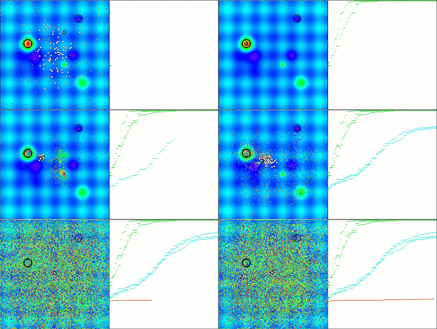
CTA on the Hilly test function
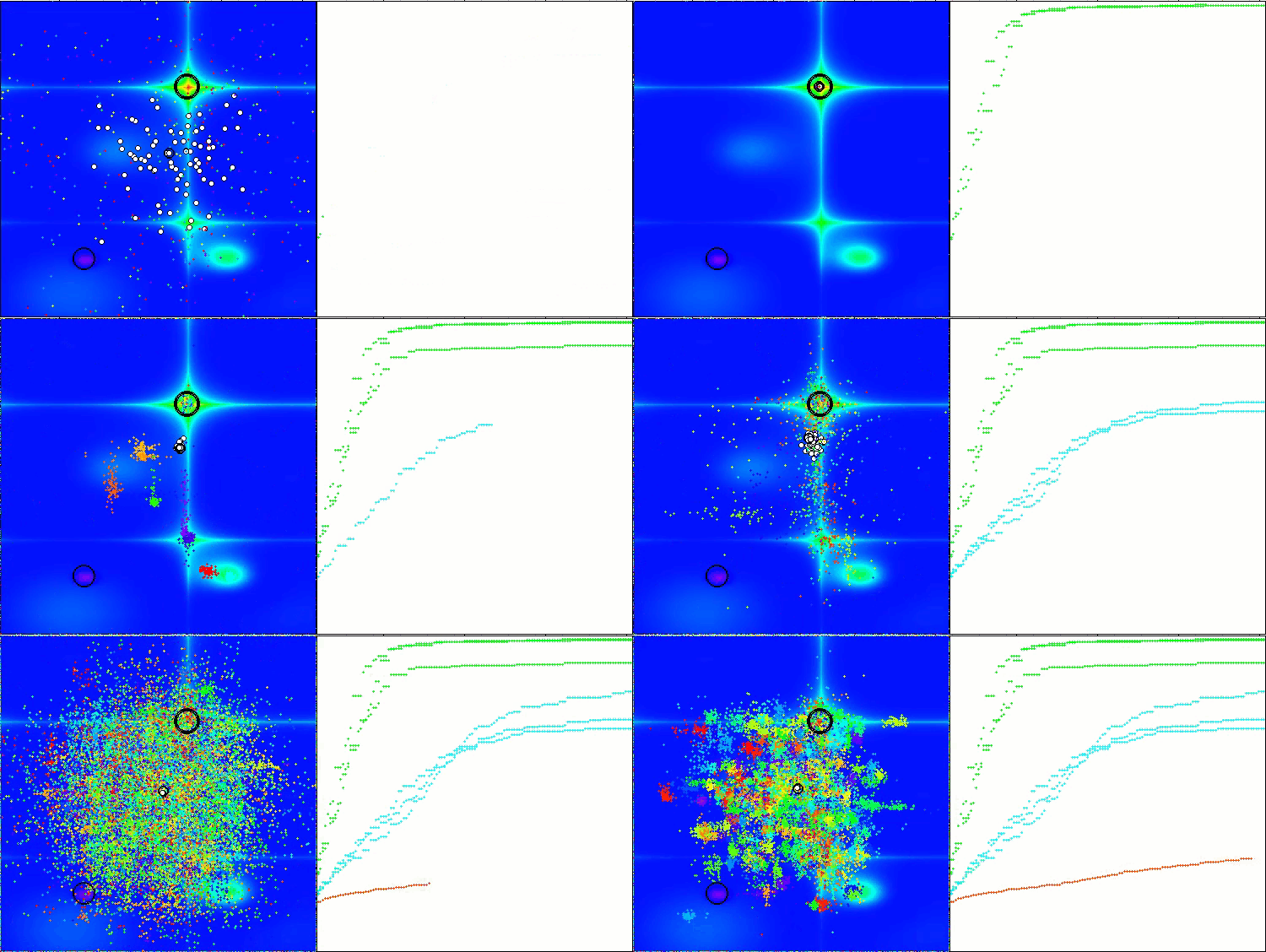
CTA on the Forest test function
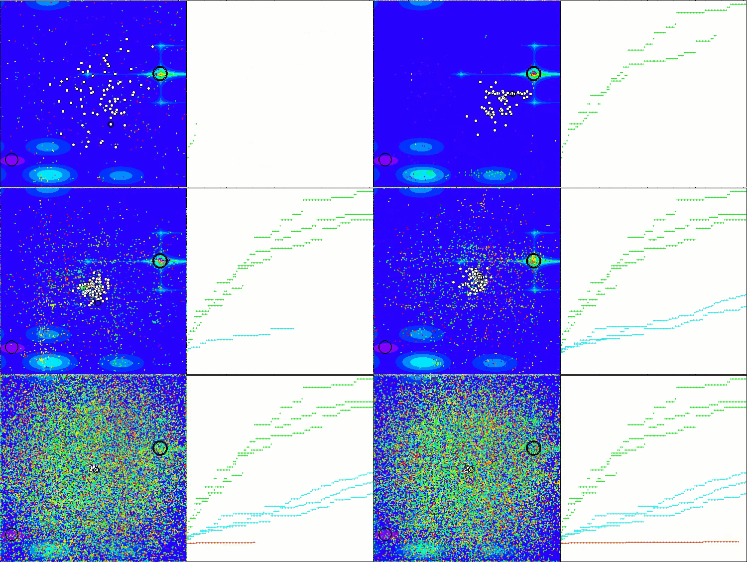
CTA on the Megacity test function
Based on the test results, the CTA algorithm occupies a worthy 3rd place in the rating table.
| # | AO | Description | Hilly | Hilly final | Forest | Forest final | Megacity (discrete) | Megacity final | Final result | % of MAX | ||||||
| 10 p (5 F) | 50 p (25 F) | 1000 p (500 F) | 10 p (5 F) | 50 p (25 F) | 1000 p (500 F) | 10 p (5 F) | 50 p (25 F) | 1000 p (500 F) | ||||||||
| 1 | BGA | binary genetic algorithm | 0.99992 | 0.99484 | 0.50483 | 2.49959 | 1.00000 | 0.99975 | 0.32054 | 2.32029 | 0.90667 | 0.96400 | 0.23035 | 2.10102 | 6.921 | 76.90 |
| 2 | (P+O)ES | (P+O) evolution strategies | 0.99934 | 0.91895 | 0.56297 | 2.48127 | 1.00000 | 0.93522 | 0.39179 | 2.32701 | 0.83167 | 0.64433 | 0.21155 | 1.68755 | 6.496 | 72.18 |
| 3 | CTA | comet tail algorithm | 0.95346 | 0.86319 | 0.27770 | 2.09435 | 0.99794 | 0.85740 | 0.33949 | 2.19484 | 0.88769 | 0.56431 | 0.10512 | 1.55712 | 5.846 | 64.96 |
| 4 | SDSm | stochastic diffusion search M | 0.93066 | 0.85445 | 0.39476 | 2.17988 | 0.99983 | 0.89244 | 0.19619 | 2.08846 | 0.72333 | 0.61100 | 0.10670 | 1.44103 | 5.709 | 63.44 |
| 5 | ESG | evolution of social groups | 0.99906 | 0.79654 | 0.35056 | 2.14616 | 1.00000 | 0.82863 | 0.13102 | 1.95965 | 0.82333 | 0.55300 | 0.04725 | 1.42358 | 5.529 | 61.44 |
| 6 | SIA | simulated isotropic annealing | 0.95784 | 0.84264 | 0.41465 | 2.21513 | 0.98239 | 0.79586 | 0.20507 | 1.98332 | 0.68667 | 0.49300 | 0.09053 | 1.27020 | 5.469 | 60.76 |
| 7 | TSEA | turtle shell evolution algorithm | 0.96798 | 0.64480 | 0.29672 | 1.90949 | 0.99449 | 0.61981 | 0.22708 | 1.84139 | 0.69077 | 0.42646 | 0.13598 | 1.25322 | 5.004 | 55.60 |
| 8 | DE | differential evolution | 0.95044 | 0.61674 | 0.30308 | 1.87026 | 0.95317 | 0.78896 | 0.16652 | 1.90865 | 0.78667 | 0.36033 | 0.02953 | 1.17653 | 4.955 | 55.06 |
| 9 | BSA | bird swarm algorithm | 0.90857 | 0.73661 | 0.25767 | 1.90285 | 0.90437 | 0.81619 | 0.16401 | 1.88457 | 0.61692 | 0.54154 | 0.10951 | 1.26797 | 5.055 | 56.17 |
| 10 | HS | harmony search | 0.86509 | 0.68782 | 0.32527 | 1.87818 | 0.99999 | 0.68002 | 0.09590 | 1.77592 | 0.62000 | 0.42267 | 0.05458 | 1.09725 | 4.751 | 52.79 |
| 11 | SSG | saplings sowing and growing | 0.77839 | 0.64925 | 0.39543 | 1.82308 | 0.85973 | 0.62467 | 0.17429 | 1.65869 | 0.64667 | 0.44133 | 0.10598 | 1.19398 | 4.676 | 51.95 |
| 12 | (PO)ES | (PO) evolution strategies | 0.79025 | 0.62647 | 0.42935 | 1.84606 | 0.87616 | 0.60943 | 0.19591 | 1.68151 | 0.59000 | 0.37933 | 0.11322 | 1.08255 | 4.610 | 51.22 |
| 13 | BSO | brain storm optimization | 0.91301 | 0.56222 | 0.30047 | 1.77570 | 0.97162 | 0.57162 | 0.23449 | 1,77772 | 0.60462 | 0.27138 | 0.12011 | 0.99611 | 4.550 | 50.55 |
| 14 | WOAm | wale optimization algorithm M | 0.84521 | 0.56298 | 0.26263 | 1.67081 | 0.93100 | 0.52278 | 0.16365 | 1.61743 | 0.66308 | 0.41138 | 0.11357 | 1.18803 | 4.476 | 49.74 |
| 15 | ACOm | ant colony optimization M | 0.88190 | 0.66127 | 0.30377 | 1.84693 | 0.85873 | 0.58680 | 0.15051 | 1.59604 | 0.59667 | 0.37333 | 0.02472 | 0.99472 | 4.438 | 49.31 |
| 16 | BFO-GA | bacterial foraging optimization - ga | 0.89150 | 0.55111 | 0.31529 | 1.75790 | 0.96982 | 0.39612 | 0.06305 | 1.42899 | 0.72667 | 0.27500 | 0.03525 | 1.03692 | 4.224 | 46.93 |
| 17 | MEC | mind evolutionary computation | 0.69533 | 0.53376 | 0.32661 | 1.55569 | 0.72464 | 0.33036 | 0.07198 | 1.12698 | 0.52500 | 0.22000 | 0.04198 | 0.78698 | 3.470 | 38.55 |
| 18 | IWO | invasive weed optimization | 0.72679 | 0.52256 | 0.33123 | 1.58058 | 0.70756 | 0.33955 | 0.07484 | 1.12196 | 0.42333 | 0.23067 | 0.04617 | 0.70017 | 3.403 | 37.81 |
| 19 | Micro-AIS | micro artificial immune system | 0.79547 | 0.51922 | 0.30861 | 1.62330 | 0.72956 | 0.36879 | 0.09398 | 1.19233 | 0.37667 | 0.15867 | 0.02802 | 0.56335 | 3.379 | 37.54 |
| 20 | COAm | cuckoo optimization algorithm M | 0.75820 | 0.48652 | 0.31369 | 1.55841 | 0.74054 | 0.28051 | 0.05599 | 1.07704 | 0.50500 | 0.17467 | 0.03380 | 0.71347 | 3.349 | 37.21 |
| 21 | SDOm | spiral dynamics optimization M | 0.74601 | 0.44623 | 0.29687 | 1.48912 | 0.70204 | 0.34678 | 0.10944 | 1.15826 | 0.42833 | 0.16767 | 0.03663 | 0.63263 | 3.280 | 36.44 |
| 22 | NMm | Nelder-Mead method M | 0.73807 | 0.50598 | 0.31342 | 1.55747 | 0.63674 | 0.28302 | 0.08221 | 1.00197 | 0.44667 | 0.18667 | 0.04028 | 0.67362 | 3.233 | 35.92 |
| 23 | FAm | firefly algorithm M | 0.58634 | 0.47228 | 0.32276 | 1.38138 | 0.68467 | 0.37439 | 0.10908 | 1.16814 | 0.28667 | 0.16467 | 0.04722 | 0.49855 | 3.048 | 33.87 |
| 24 | GSA | gravitational search algorithm | 0.64757 | 0.49197 | 0.30062 | 1.44016 | 0.53962 | 0.36353 | 0.09945 | 1.00260 | 0.32667 | 0.12200 | 0.01917 | 0.46783 | 2.911 | 32.34 |
| 25 | BFO | bacterial foraging optimization | 0.61171 | 0.43270 | 0.31318 | 1.35759 | 0.54410 | 0.21511 | 0.05676 | 0.81597 | 0.42167 | 0.13800 | 0.03195 | 0.59162 | 2.765 | 30.72 |
| 26 | ABC | artificial bee colony | 0.63377 | 0.42402 | 0.30892 | 1.36671 | 0.55103 | 0.21874 | 0.05623 | 0.82600 | 0.34000 | 0.14200 | 0.03102 | 0.51302 | 2.706 | 30.06 |
| 27 | BA | bat algorithm | 0.59761 | 0.45911 | 0.35242 | 1.40915 | 0.40321 | 0.19313 | 0.07175 | 0.66810 | 0.21000 | 0.10100 | 0.03517 | 0.34617 | 2.423 | 26.93 |
| 28 | SA | simulated annealing | 0.55787 | 0.42177 | 0.31549 | 1.29513 | 0.34998 | 0.15259 | 0.05023 | 0.55280 | 0.31167 | 0.10033 | 0.02883 | 0.44083 | 2.289 | 25.43 |
| 29 | IWDm | intelligent water drops M | 0.54501 | 0.37897 | 0.30124 | 1.22522 | 0.46104 | 0.14704 | 0.04369 | 0.65177 | 0.25833 | 0.09700 | 0.02308 | 0.37842 | 2.255 | 25.06 |
| 30 | PSO | particle swarm optimisation | 0.59726 | 0.36923 | 0.29928 | 1.26577 | 0.37237 | 0.16324 | 0.07010 | 0.60572 | 0.25667 | 0.08000 | 0.02157 | 0.35823 | 2.230 | 24.77 |
| 31 | Boids | boids algorithm | 0.43340 | 0.30581 | 0.25425 | 0.99346 | 0.35718 | 0.20160 | 0.15708 | 0.71586 | 0.27846 | 0.14277 | 0.09834 | 0.51957 | 2.229 | 24.77 |
| 32 | MA | monkey algorithm | 0.59107 | 0.42681 | 0.31816 | 1.33604 | 0.31138 | 0.14069 | 0.06612 | 0.51819 | 0.22833 | 0.08567 | 0.02790 | 0.34190 | 2.196 | 24.40 |
| 33 | SFL | shuffled frog-leaping | 0.53925 | 0.35816 | 0.29809 | 1.19551 | 0.37141 | 0.11427 | 0.04051 | 0.52618 | 0.27167 | 0.08667 | 0.02402 | 0.38235 | 2.104 | 23.38 |
| 34 | FSS | fish school search | 0.55669 | 0.39992 | 0.31172 | 1.26833 | 0.31009 | 0.11889 | 0.04569 | 0.47467 | 0.21167 | 0.07633 | 0.02488 | 0.31288 | 2.056 | 22.84 |
| 35 | RND | random | 0.52033 | 0.36068 | 0.30133 | 1.18234 | 0.31335 | 0.11787 | 0.04354 | 0.47476 | 0.25333 | 0.07933 | 0.02382 | 0.35648 | 2.014 | 22.37 |
| 36 | GWO | grey wolf optimizer | 0.59169 | 0.36561 | 0.29595 | 1.25326 | 0.24499 | 0.09047 | 0.03612 | 0.37158 | 0.27667 | 0.08567 | 0.02170 | 0.38403 | 2.009 | 22.32 |
| 37 | CSS | charged system search | 0.44252 | 0.35454 | 0.35201 | 1.14907 | 0.24140 | 0.11345 | 0.06814 | 0.42299 | 0.18333 | 0.06300 | 0.02322 | 0.26955 | 1.842 | 20.46 |
| 38 | EM | electroMagnetism-like algorithm | 0.46250 | 0.34594 | 0.32285 | 1.13129 | 0.21245 | 0.09783 | 0.10057 | 0.41085 | 0.15667 | 0.06033 | 0.02712 | 0.24412 | 1.786 | 19.85 |
Summary
The considered CTA algorithm is based on the concept of cometary motion and has a number of features that contradict the physical laws and evolution of comets. The impact of these features on the final results of the algorithm should be considered in more detail.
One of the contradictions concerns the direction of the comet's tail. In the CTA algorithm, using the tail direction towards the star (Dir_P = -1) generally improves its performance significantly. However, using the direction of the star's tail also improves the algorithm's ability to explore space. Optimization enthusiasts may wish to consider using a dynamic tail direction coefficient depending on the current epoch. It is worth noting that the direction of the tail away from the star provides better convergence on low-dimensional problems, while the direction towards the star is more effective on high-dimensional problems.
Another controversy is the size of the comet's tail. In the CTA algorithm, it was found that dynamically changing the tail size (increasing it with increasing distance to the star) improves the efficiency of the algorithm. This contradicts the laws of physics, since in reality the size of a comet's tail increases as it approaches the Sun. However, such a dynamic change in the tail size allows us to expand the area of study of the solution space around the comet nucleus in remote areas from the global solution, increasing the chances of discovering promising solutions and reducing the likelihood of getting stuck in local extremes. As it approaches the star, the comet's tail decreases, which increases the intensity of the solution refinement.
The CTA algorithm also involves the exchange of information between comets, similar to what happens in nature when comets capture particles left behind by other comets. This is an additional feature of the algorithm for exploring the solution space. Attempts have been made to use methods to increase population diversity by modeling coronal mass ejections from the star and by exploiting the combinatorial properties of the algorithm by borrowing the coordinates of some comets from others.
CTA (Comet Tail Algorithm) is an interesting new approach to optimization that uses the concept of comet movement. The algorithm demonstrates good convergence on various types of functions (both smooth and discrete), is very easy to implement (the structure of the algorithm is very simple, which simplifies its software implementation), does not require significant computing resources (since it does not use sorting of solutions and does not use calculations of distances between all solutions, which allows it to be used on a wide range of problems), demonstrates a small spread of results on discrete functions (stability and reproducibility of results when working with discrete target functions, as in most problems of optimization of trading systems), but at the same time the algorithm has many external parameters (such as the size of the comet tail, coefficients of tail and direction shift, etc.). On smooth functions of high dimension, the algorithm may not show the highest results.
In general, the CTA peculiarities lie in the dynamic balance between the exploration of the solution space and the refinement of the found global optimum.
Thus, the CTA algorithm uses a number of simplifications and assumptions that do not fully correspond to the physical laws of cometary motion. However, these deviations from reality allow us to increase the efficiency of the algorithm in solving optimization problems while maintaining the simplicity of implementation.
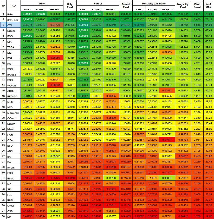
Figure 3. Color gradation of algorithms according to relevant tests Results greater than or equal to 0.99 are highlighted in white
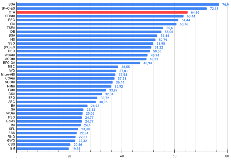
Figure 4. The histogram of algorithm test results (on a scale from 0 to 100, the more the better,
where 100 is the maximum possible theoretical result, the archive features a script for calculating the rating table)
CTA pros and cons:
Advantages:
- Good convergence on various types of functions.
- Simple implementation.
- Undemanding to computing resources.
- Small scatter of results on discrete functions.
Disadvantages:
- Many external parameters.
- Poor results on smooth high-dimensional functions.
Source codes
The article is accompanied by an archive with the current versions of the algorithm codes. The author of the article is not responsible for the absolute accuracy in the description of canonical algorithms. Changes have been made to many of them to improve search capabilities. The conclusions and judgments presented in the articles are based on the results of the experiments.
Translated from Russian by MetaQuotes Ltd.
Original article: https://www.mql5.com/ru/articles/14841
 Multiple Symbol Analysis With Python And MQL5 (Part I): NASDAQ Integrated Circuit Makers
 Reimagining Classic Strategies in MQL5 (Part III): FTSE 100 Forecasting
 How to develop any type of Trailing Stop and connect it to an EA
 Gain An Edge Over Any Market (Part IV): CBOE Euro And Gold Volatility Indexes
- Free trading apps
- Over 8,000 signals for copying
- Economic news for exploring financial markets
You agree to website policy and terms of use