Multiple Symbol Analysis With Python And MQL5 (Part I): NASDAQ Integrated Circuit Makers

There are many ways for an investor to diversify their portfolio. Furthermore, there are many different metrics to be used as a criterion for how well the portfolio has been optimized. It is unlikely, that any single investor will have ample time or resources to carefully consider all their options before committing to such a big decision. In this series of articles, we will walk you through the myriad of options that lie ahead of you in your journey to trade multiple symbols simultaneously. Our goal is to help you decide which strategies to keep and which ones may not suitable for you.

Overview of The Trading Strategy

In this discussion, we have selected a basket of stocks that are fundamentally related to each other. We have selected 5 stocks of companies that design and sell integrated circuits in their business cycle. These companies are Broadcom, Cisco, Intel, NVIDIA and Comcast. All 5 companies are listed on the National Association of Securities Dealers Automated Quotations (NASDAQ) Exchange. NASDAQ was established in 1971 and is the largest exchange in the United States by trading volume.

Integrated circuits have become a staple of our everyday life. These electronic chips permeate all aspects of our modern lives, from the proprietary MetaQuotes servers that host this very website that you are reading this article on, down to the device you are using to read this article all these devices rely on technology that is most likely developed by one of these 5 companies. The world’s first integrated circuit was developed by Intel, it was branded the Intel 4004, and was launched in 1971, the same year the NASDAQ exchange was founded. The Intel 4004 had approximately, 2600 transistors, a far-cry from modern chips that easily have billions of transistors.

Since we are motivated by the global demand for integrated circuits, we desire to intelligently gain exposure to the chip market. Given a basket of these 5 stocks, we will demonstrate how to maximize the return of your portfolio by prudently allocating capital between them. A traditional approach of uniform distribution of capital between all 5 stocks will not suffice in modern, volatile markets. We will instead build a model that informs us whether we should buy or sell each stock, and the optimal quantities we should trade. In other words, we are using the data we have at hand to algorithmically learn our position sizing and quantities.

Overview of The Methodology

We began by fetching 100000 rows of M1 market data for each of the 5 stocks in our basket, from our MetaTrader 5 Terminal using the MetaTrader 5 Python library. After converting the ordinary price data to percent changes, we performed exploratory data analysis on the market returns data.

We observed feeble correlation levels between the 5 stocks. Furthermore, our box-plots clearly showed that the average return from each stock was close to 0. We also plotted the returns from each stock in an overlaid fashion, and we could clearly observe that NVIDIA stock returns appeared the most volatile. Lastly, we created pair plots across all 5 stocks we have selected, and unfortunately, we could not observe any discernible relationship we could advantage of.

From there, we used the SciPy library to find optimal weights for each of our 5 stocks in our portfolio. We will permit all the 5 weights to range between -1 and 1. Whenever our portfolio weight is below 0, the algorithm is telling us to sell and conversely, when our weights are above 0, the data is suggesting we buy.

After calculating the optimal portfolio weights, we integrated this data into our trading application to ensure that it always maintained an optimal number of positions open in each market. Our trading application is designed to close any open positions automatically if they reach a profit level, specified by the end user.

Fetching The Data 

To get started, let us first import the libraries we need.

#Import the libraries we need
import pandas              as pd
import numpy               as np
import seaborn             as sns
import matplotlib.pyplot   as plt
import MetaTrader5         as mt5
from   scipy.optimize      import minimize

Now let us initialize the MetaTrader 5 terminal.

#Initialize the terminal
mt5.initialize()

True

Define the basket of stocks we wish to trade.

#Now let us fetch the data we need on chip manufacturing stocks
#Broadcom, Cisco, Comcast, Intel, NVIDIA
stocks = ["AVGO.NAS","CSCO.NAS","CMCSA.NAS","INTC.NAS","NVDA.NAS"]

Let us create a data-frame to store our market data.

#Let us create a data frame to store our stock returns
amount = 100000
returns = pd.DataFrame(columns=stocks,index=np.arange(0,amount))

Now, we will fetch our market data.

#Fetch the stock returns
for stock in stocks:
    temp = pd.DataFrame(mt5.copy_rates_from_pos(stock,mt5.TIMEFRAME_M1,0,amount))
    returns[[stock]] = temp[["close"]].pct_change()

Let us format our data.

#Format the data set 
returns.dropna(inplace=True)
returns.reset_index(inplace=True,drop=True)
returns

Finally, multiply the data by 100 to save it as percentages.

#Convert the returns to percentages
returns = returns * 100
returns

Exploratory Data Analysis

Sometimes, we can visually see the relationship between the variables in the system. Let us analyze the correlation levels in our data to see if there are any linear combinations we can take advantage of. Unfortunately, our correlation levels our not impressive and so far, there appears to be no linear dependencies for us to exploit.

#Let's analyze if there is any correlation in the data
sns.heatmap(returns.corr(),annot=True)

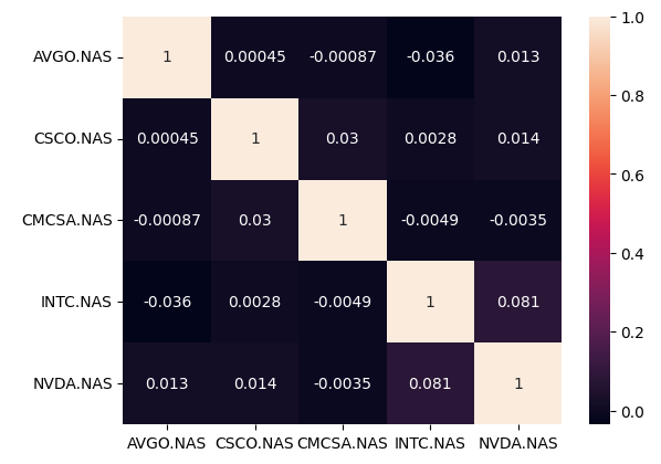
Fig 1: Our correlation heat-map

Let us analyze pair-wise scatter-plots of our data. When dealing with large data-sets, non-trivial relationships may easily slip past us undetected. Pair-wise plots will minimize the chances of this happening. Unfortunately, there were no easily observable relationships in the data that were revealed to us by our plots.

#Let's create pair plots of our data
sns.pairplot(returns)

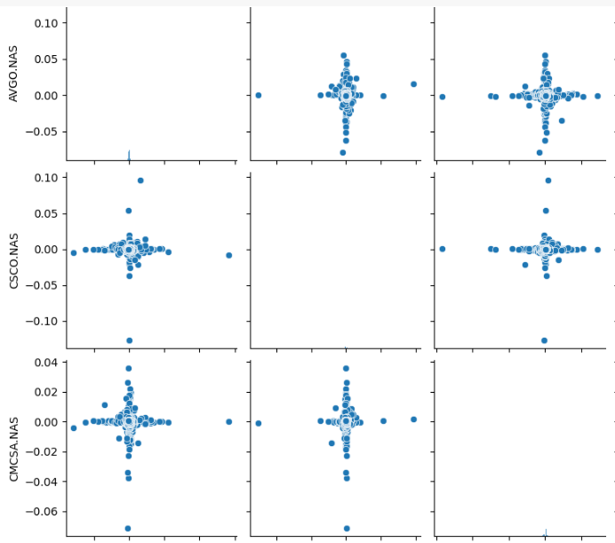
Fig 2: Some of our pair-wise scatter-plots

Plotting the returns we observed in the data shows us that NVIDIA appears to have the most volatile returns.

#Lets also visualize our returns
returns.plot()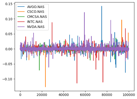

Fig 3: Plotting our market returns

Visualizing our market returns as box-plots clearly shows us that the average market return is 0.

#Let's try creating box-plots 
sns.boxplot(returns)

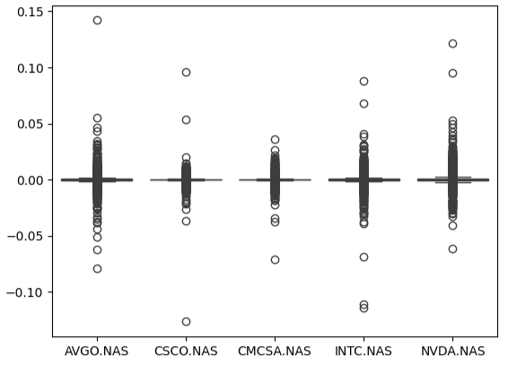
Fig 4: Visualizing our market returns as box-plots

Portfolio Optimization

We are now ready to start calculating optimal weights of capital allocation for each stock. Initially, we will assign our weights randomly. Furthermore, we will also create a data-structure to store the progress of our optimization algorithm.

#Define random weights that add up to 1
weights = np.array([1,0.5,0,0.5,-1])
#Create a data structure to store the progress of the algorithm
evaluation_history = []

The objective function of our optimization procedure will be the return of our portfolio under the given weights. Note that, our portfolio returns will be calculated using the geometric mean of the asset returns. We chose to employ the geometric mean over the arithmetic mean because, when dealing with positive and negative values, calculating the mean is no longer a trivial task. If we approached this problem casually and employed the arithmetic mean, we could've easily calculated a portfolio return of 0. We can use minimization algorithms for maximization problems by multiplying the portfolio return by negative 1 before returning it to the optimization algorithm.

#Let us now get ready to maximize our returns
#First we need to define the cost function
def cost_function(x):
    #First we need to calculate the portfolio returns with the suggested weights
    portfolio_returns = np.dot(returns,x)
    geom_mean         =  ((np.prod( 1 + portfolio_returns ) ** (1.0/99999.0)) - 1)
    #Let's keep track of how our algorithm is performing
    evaluation_history.append(-geom_mean)
    return(-geom_mean)

Let us now define the constraint that ensures all our weights add up to 1. Note that only a few optimization procedures in SciPy support equality constraints. Equality constraints inform the SciPy module that we would like for this function to equate to 0. Therefore, we want the difference between the absolute value of our weights and 1 to be 0.

#Now we need to define our constraints
def l1_norm_constraint(x):
    return(((np.sum(np.abs(x))) - 1))

constraints = ({'type':'eq','fun':l1_norm_constraint})

All our weights should be between -1 and 1. This can be enforced by defining bounds for our algorithm.

#Now we need to define the bounds for our weights
bounds = [(-1,1)] * 5

Performing the optimization procedure.

#Perform the optimization
results = minimize(cost_function,weights,method="SLSQP",bounds=bounds,constraints=constraints)

The results of our optimization procedure.

results

message: Optimization terminated successfully
 success: True
  status: 0
     fun: 0.0024308603411499208
       x: [ 3.931e-01  1.138e-01 -5.991e-02  7.744e-02 -3.557e-01]
     nit: 23
     jac: [ 3.851e-04  2.506e-05 -3.083e-04 -6.868e-05 -3.186e-04]
    nfev: 158
    njev: 23

Let us store the optimal coefficient values we calculated.

optimal_weights = results.x
optimal_weights

array([ 0.39311134,  0.11379942, -0.05991417,  0.07743534, -0.35573973])

We should also store the optimal points from the procedure.

optima_y = min(evaluation_history)
optima_x = evaluation_history.index(optima_y)
inputs = np.arange(0,len(evaluation_history))

Let us visualize the performance history of our optimization algorithm. As we can see from the plot, our algorithm appears to have struggled in the beginning over the first 50 iterations. However, it appears to have been able to find an optimal point that maximizes our portfolio returns.

plt.scatter(inputs,evaluation_history)
plt.plot(optima_x,optima_y,'s',color='r')
plt.axvline(x=optima_x,ls='--',color='red')
plt.axhline(y=optima_y,ls='--',color='red')
plt.title("Maximizing Returns")

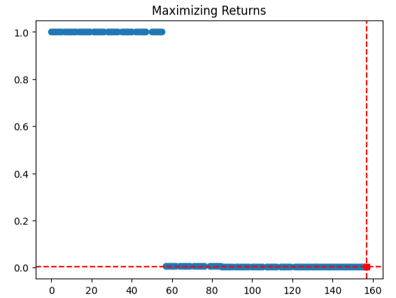
Fig 5: Our SLSQP optimization algorithm's performance

Let us check that the absolute value of our weights add up to 1, or in other words, we wish to validate that our L1-norm constraint was not violated.

#Validate the weights add up to 1
np.sum(np.abs(optimal_weights))

1.0

There is an intuitive way we can interpret the optimal coefficients. If we assume that we want to open 10 positions, we will first multiply the coefficients by 10. Then we will perform integer division by 1 to drop off any decimal places. The integers we have left over could be interpreted as the number of positions we should open in each market. Our data appears to be suggesting that we open 3 long positions in Broadcom, 1 long position in Cisco, 1 short position in Comcast, no positions in Intel and 4 short positions in NVIDIA to maximize our returns. 

#Here's an intuitive way of understanding the data
#If we can only open 10 positions, our best bet may be
#3 buy positions in Broadcom
#1 buy position in Cisco
#1 sell position sell position in Comcast
#No positions in Intel
#4 sell postions in NVIDIA
(optimal_weights * 10) // 1

array([ 3.,  1., -1.,  0., -4.])

Implementation In MQL5

Let us now implement our trading strategy in MQL5. We will get the ball rolling by first defining global variables we will use in our application.

//+------------------------------------------------------------------+
//|                                                 NASDAQ IC AI.mq5 |
//|                                        Gamuchirai Zororo Ndawana |
//|                          https://www.mql5.com/en/gamuchiraindawa |
//+------------------------------------------------------------------+
#property copyright "Gamuchirai Zororo Ndawana"
#property link      "https://www.mql5.com/en/gamuchiraindawa"
#property version   "1.00"

//+------------------------------------------------------------------+
//| Global variables                                                 |
//+------------------------------------------------------------------+
int    rsi_handler,bb_handler;
double bid,ask;
int    optimal_weights[5] = {3,1,-1,0,-4};
string stocks[5]          = {"AVGO.NAS","CSCO.NAS","CMCSA.NAS","INTC.NAS","NVDA.NAS"};
vector current_close      = vector::Zeros(1);
vector rsi_buffer         = vector::Zeros(1);
vector bb_high_buffer     = vector::Zeros(1);
vector bb_mid_buffer      = vector::Zeros(1);
vector bb_low_buffer      = vector::Zeros(1);

Importing the trade library to help us manage our positions.

//+------------------------------------------------------------------+
//| Libraries                                                        |
//+------------------------------------------------------------------+
#include  <Trade/Trade.mqh>
CTrade Trade;

The end-user of our program can adjust the behavior of the Expert Advisor through the inputs we allow them to control.

//+------------------------------------------------------------------+
//| User inputs                                                      |
//+------------------------------------------------------------------+
input double profit_target =  1.0; //At this profit level, our position will be closed
input int    rsi_period    =   20; //Adjust the RSI period
input int    bb_period     =   20; //Adjust the Bollinger Bands period
input double trade_size    =  0.3; //How big should our trades be?

Whenever our trading algorithm is being set up for the first time, we need to ensure that all 5 symbols from our previous calculations are available to us. Otherwise, we will abort the initialization procedure.

//+------------------------------------------------------------------+
//| Expert initialization function                                   |
//+------------------------------------------------------------------+
int OnInit()
  {
//--- Validate that all the symbols we need are available
   if(!validate_symbol())
     {
      return(INIT_FAILED);
     }
//--- Everything went fine
   return(INIT_SUCCEEDED);
  }

If our program has been removed from the chart, we should free up the resources we are no longer using.

//+------------------------------------------------------------------+
//| Expert deinitialization function                                 |
//+------------------------------------------------------------------+
void OnDeinit(const int reason)
  {
//--- Release resources we no longer need
   release_resources();
  }

Whenever we receive updated prices, we would first like to store the current bid and ask in our globally defined variables, check for trading opportunities and finally take any profits we have ready off the table.

//+------------------------------------------------------------------+
//| Expert tick function                                             |
//+------------------------------------------------------------------+
void OnTick()
  {

//--- Update market data
   update_market_data();

//--- Check for a trade oppurtunity in each symbol
   check_trade_symbols();

//--- Check if we have an oppurtunity to take ourt profits
   check_profits();
  }

The function responsible for taking our profits off the table will iterate over all the symbols we have in our basket. If it can successfully find the symbol, it will check if we have any positions in that market. Assuming we have open positions, we will check if the profit surpasses the user's defined profit target, if it does, then we will close our positions. Otherwise, we will move on.

//+------------------------------------------------------------------+
//| Check for opportunities to collect our profits                   |
//+------------------------------------------------------------------+
void check_profits(void)
  {
   for(int i =0; i < 5; i++)
     {
      if(SymbolSelect(stocks[i],true))
        {
         if(PositionSelect(stocks[i]))
           {
            if(PositionGetDouble(POSITION_PROFIT) > profit_target)
              {
               Trade.PositionClose(stocks[i]);
              }
           }
        }
     }
  }

Anytime we receive updated prices, we want to store them in our globally scoped variables because these variables may be called in various parts of our program.

//+------------------------------------------------------------------+
//| Update markte data                                               |
//+------------------------------------------------------------------+
void update_market_data(void)
  {
   ask = SymbolInfoDouble(Symbol(),SYMBOL_ASK);
   bid = SymbolInfoDouble(Symbol(),SYMBOL_BID);
  }

Whenever our Expert Advisor is not in use, we will free up the resources it no longer needs to ensure a good end-user experience.

//+-------------------------------------------------------------------+
//| Release the resources we no longer need                           |
//+-------------------------------------------------------------------+
void release_resources(void)
  {
   ExpertRemove();
  }
//+------------------------------------------------------------------+

Upon initialization, we checked if all the symbols we required are available. The function below is responsible for that task. It iterates over all the symbols we have in our array of stocks. If we fail to select any symbol, the function will return false, and halt the initialization procedure. Otherwise, the function will return true.

//+------------------------------------------------------------------+
//| Validate that all the symbols we need are available              |
//+------------------------------------------------------------------+
bool validate_symbol(void)
  {
   for(int i=0; i < 5; i++)
     {
      //--- We failed to add one of the necessary symbols to the Market Watch window!
      if(!SymbolSelect(stocks[i],true))
        {
         Comment("Failed to add ",stocks[i]," to the market watch. Ensure the symbol is available.");
         return(false);
        }
     }

//--- Everything went fine
   return(true);
  }

This function is responsible for coordinating the process of opening and managing positions in our portfolio. It will iterate through all the symbols in our array and check if we have open positions in that market and if we should have open positions in that market. If we should, but we do not, the function will start the process of checking for opportunities to gain exposure in that market. Otherwise, the function will do nothing.

//+------------------------------------------------------------------+
//| Check if we have any trade opportunities                         |
//+------------------------------------------------------------------+
void check_trade_symbols(void)
  {
//--- Loop through all the symbols we have
   for(int i=0;i < 5;i++)
     {
      //--- Select that symbol and check how many positons we have open
      if(SymbolSelect(stocks[i],true))
        {
         //--- If we have no positions in that symbol, optimize the portfolio
         if((PositionsTotal() == 0) && (optimal_weights[i] != 0))
           {
            optimize_portfolio(stocks[i],optimal_weights[i]);
           }
        }
     }
  }

The optimize portfolio function takes 2 parameters, the stock under question and the weights attributed to that stock. If the weights are positive, the function will call initiate a procedure to assume a long position in that market until the weight parameter has been met, the opposite is true for negative weights.

//+------------------------------------------------------------------+
//| Optimize our portfolio                                           |
//+------------------------------------------------------------------+
void optimize_portfolio(string symbol,int weight)
  {
//--- If the weight is less than 0, check if we have any oppurtunities to sell that stock
   if(weight < 0)
     {
      if(SymbolSelect(symbol,true))
        {
         //--- If we have oppurtunities to sell, act on it
         if(check_sell(symbol, weight))
           {
            Trade.Sell(trade_size,symbol,bid,0,0,"NASDAQ IC AI");
           }
        }
     }

//--- Otherwise buy
   else
     {
      if(SymbolSelect(symbol,true))
        {
         //--- If we have oppurtunities to buy, act on it
         if(check_buy(symbol,weight))
           {
            Trade.Buy(trade_size,symbol,ask,0,0,"NASDAQ IC AI");
           }
        }
     }
  }

Now we must define the conditions under which we can enter a long position. We will rely on a combination of technical analysis and price action to time our entries. We will only enter long positions if price levels are above the uppermost Bollinger Band, our RSI levels are above 70 and price action on higher time-frames has been bullish. Likewise, we believe that this may constitute a high probability setup, which would allow us to achieve our profit targets, safely. Lastly, our final condition is that the total number of positions we have open in that market, do not exceed our optimal allocation levels. If our conditions are satisfied, then we will return true, which will give the "optimize_portfolio" function authorization to enter a long position.

//+------------------------------------------------------------------+
//| Check for oppurtunities to buy                                   |
//+------------------------------------------------------------------+
bool check_buy(string symbol, int weight)
  {
//--- Ensure we have selected the right symbol
   SymbolSelect(symbol,true);

//--- Load the indicators on the symbol
   bb_handler  = iBands(symbol,PERIOD_CURRENT,bb_period,0,1,PRICE_CLOSE);
   rsi_handler = iRSI(symbol,PERIOD_CURRENT,rsi_period,PRICE_CLOSE);
//--- Validate the indicators
   if((bb_handler == INVALID_HANDLE) || (rsi_handler == INVALID_HANDLE))
     {
      //--- Something went wrong
      return(false);
     }

//--- Load indicator readings into the buffers
   bb_high_buffer.CopyIndicatorBuffer(bb_handler,1,0,1);
   rsi_buffer.CopyIndicatorBuffer(rsi_handler,0,0,1);
   current_close.CopyRates(symbol,PERIOD_CURRENT,COPY_RATES_CLOSE,0,1);

//--- Validate that we have a valid buy oppurtunity
   if((bb_high_buffer[0] < current_close[0]) && (rsi_buffer[0] > 70))
     {
      return(false);
     }

//--- Do we allready have enough positions
   if(PositionsTotal() >= weight)
     {
      return(false);
     }
//--- We can open a position
   return(true);
  }

Our "check_sell" function works similarly to our check buy function, except that it multiplies the weight by negative 1 first so that we can easily count how many positions we should have open in the market. The function will proceed to check if price is beneath the Bollinger Band Low and that the RSI reading is less than 30. If these 3 conditions are met, we also need to ensure that the price action on higher time frames permits us to enter a short position.

//+------------------------------------------------------------------+
//| Check for oppurtunities to sell                                  |
//+------------------------------------------------------------------+
bool check_sell(string symbol, int weight)
  {
//--- Ensure we have selected the right symbol
   SymbolSelect(symbol,true);

//--- Negate the weight
   weight = weight * -1;

//--- Load the indicators on the symbol
   bb_handler  = iBands(symbol,PERIOD_CURRENT,bb_period,0,1,PRICE_CLOSE);
   rsi_handler = iRSI(symbol,PERIOD_CURRENT,rsi_period,PRICE_CLOSE);
//--- Validate the indicators
   if((bb_handler == INVALID_HANDLE) || (rsi_handler == INVALID_HANDLE))
     {
      //--- Something went wrong
      return(false);
     }

//--- Load indicator readings into the buffers
   bb_low_buffer.CopyIndicatorBuffer(bb_handler,2,0,1);
   rsi_buffer.CopyIndicatorBuffer(rsi_handler,0,0,1);
   current_close.CopyRates(symbol,PERIOD_CURRENT,COPY_RATES_CLOSE,0,1);

//--- Validate that we have a valid sell oppurtunity
   if(!((bb_low_buffer[0] > current_close[0]) && (rsi_buffer[0] < 30)))
     {
      return(false);
     }

//--- Do we have enough trades allready open?
   if(PositionsTotal() >= weight)
     {
      //--- We have a valid sell setup
      return(false);
     }

//--- We can go ahead and open a position
   return(true);
  }

Fig 6: Forward-testing our algorithm

Conclusion

In our discussion, we have demonstrated how you can algorithmically determine your position sizing and capital allocation using AI. There are many different aspects of a portfolio that we can optimize, like the risk (variance) of a portfolio, the correlation of our portfolio with the performance of an industry benchmark (beta) and the risk adjusted-returns of the portfolio. In our example, we kept our model simple and only considered maximizing the return. We will consider many important metrics as we progress in this series. However, this simple example allows us to grasp the main ideas behind portfolio optimization and when we even progress to arrive at complex optimization procedures, the reader can address the problem with confidence knowing that the main ideas we have outlined here won't change. While we cannot guarantee that the information contained in our discussion will generate success every time, it is certainly worth considering if you are serious about trading multiple symbols in an algorithmic fashion.