
Gain An Edge Over Any Market (Part IV): CBOE Euro And Gold Volatility Indexes

In the age of big data, there are hundreds of millions of datasets that each hold the potential to yield untapped levels of accuracy when forecasting financial markets. Unfortunately, it is unlikely that all existing datasets will live up to this potential. In this series of articles, our goal is to help you traverse the vast landscape of possible datasets and at the end of the discussion you will be well positioned to arrive at an informed on whether the suggested alternative data should be included in your trading strategy, or if you may be better off without it.
Overview of The Trading Strategy
We will analyze the XAUEUR market. The symbol tracks the price of gold in Euros. Gold is mined on every continent on Earth, except Antarctica. A significant proportion of the world’s gold is traded by the London Bullion Market Association (LBMA) to set a globally recognized benchmark for the price of gold. The Chicago Board of Options Exchange (CBOE) is an American company that provides global market infrastructure. CBOE employ their networks to create volatility indexes tracking major markets around the world. We will analyze 2 of the CBOE’s volatility indexes that track the Euro and gold markets, respectively.
Over the years, traders have realized various strategies to successfully trade volatile markets, while minimizing risk. Generally, when markets are volatile, traders stand to realize profit targets possibly in relatively short periods of time. On the other hand, it is also possible to lose significant amounts of capital rapidly, due to large gaps in price levels that may not trigger stop loss orders in a timely fashion.
Loosely speaking, some traders prefer to open fewer positions, or risk less capital than they normally would over a larger number of positions to potentially gain from profitable price moves, while minimizing their market exposure. In general, seasoned traders in volatile markets tend to take their profits a lot quicker than they would when trading quieter markets. Other traders wait for price levels to first get caught in a range between support and resistance levels. When price levels finally breakout off the range, traders may open their positions anticipating stronger moves out of the identifiable range.
Under normal market conditions, a breakout from a support and resistance zone may quickly lose momentum and begin drifting. However, when market conditions are volatile, breakouts can be followed by violent price changes in the same direction, giving traders who follow such strategies above-average returns. Regrettably, such strategies are prone to false breakouts that may violently reverse, leaving some traders in unfavorable positions holding material losses.
Overview of The Methodology
We utilized the Federal Reserve Economic Database (FRED) Python API, maintained by The St. Louis Federal Reserve, to retrieve the CBOE Euro and gold volatility economic time-series. The data is provided in daily format and contained missing values.
Unfortunately, none of the descriptions provided with the datasets explain any of the missing values. Therefore, we mean imputed all the missing values in both datasets.
In our MetaTrader 5 Terminal, we fetched approximately 4000 rows of daily market quotes on the open, high, low and close (OHLC) price of the XAUEUR symbol, using a customized script we wrote in MQL5.
When we analyzed the correlation between the CBOE alternative data and the MetaTrader 5 market data, we observed correlation levels not significantly far from 0. Notably, the correlation levels between the two alternative datasets was 0.4. Positive correlation level may suggest the presence of interactions or common market participants affecting the two markets.
When we performed scatter plots of the data, using either of the alternative datasets on the x-axis and the close price of the XAUEUR on the y-axis, there appeared to be a threshold of high volatility levels that consistently resulted in increased price levels. Regrettably, our small dataset, a total of approximately 3000 rows after merging with the alternative datasets, may be a good reason to be cautious of being misled into seeing patterns in the data that simply aren’t present.
Effectively viewing high dimensional data can be challenging. Therefore, we employed a 2-fold procedure to view our data. Initially, we created 3D scatter plots using the 2 CBOE data sets on the x and y-axis respectively, and the XAUEUR close on the z-axis. The cluster of bull candles we observed in our 2D scatter plots was still clearly visible.
Lastly, we can always take advantage of algorithms that are designed to map high dimensional data down to a lower dimensional subspace. A well-known dimensionality reduction algorithm is Principal Components Analysis. We chose to use the scikit-learn implementation of t-distributed stochastic neighbor embedding (t-SNE), to create a 2-dimensional representation of our 6-dimensional dataset. The resulting plot suggested there may be 4 distinct clusters in our dataset. Furthermore, we observed what appears to be the effect of serial dependency in our dataset, suggesting there may be a relationship evolving between our CBOE and MetaTrader 5 data sets.
The final visualization technique we used were autocorrelation plots. All the autocorrelation plots we created exhibited strong tails, this may suggest there is long-term data persisting in our time-series. This may be created by strong trends or seasonal effects. Our partial-autocorrelation plots suggested that only a few number of lags accounted for most of the autocorrelation we observed. This suggests that the time-series data may be successfully modelled as a moving average model.
After visualizing our data, we created 3 sets of predictors:
- OHLC MetaTrader 5 market data
- FRED CBOE alternative data sets
- A superset of the previous two sets
Three Identical deep neural networks were employed to compare the 3 set of predictors using 5-fold time-series cross-validation without random shuffling. The last set of predictors generated the lowest error rate when forecasting the future close price of the XAUEUR symbol. This may suggest to us that there are relationships between the two datasets that are helping our model.
Riding on the confidence of our first test, we attempted to assess the global feature importance of our deep neural network. We selected the Accumulated Local Effects (ALE) and Shapley Additive Explanations (SHAP) methods to gain insight into which models our model depends on the most. Neither of the methods we employed rejected the alternative datasets we have selected.
We tuned the hyperparameters of our model on the training set, in a 2-step process that created 2 models. Initially, we performed 500 iterations of a random search over a selection of our model parameters. In the second step, we optimized the best values of the continuous parameters of our model from the random search, using the Limited Memory Broyden Fletcher Goldfarb Shano (L-BFGS-B) algorithm. All the remaining model parameters, that were not continuous, were fixed in the second phase.
Both the customized models outperformed the default neural network on validation data. However, the model obtained by random search performed best on the test set. This indicates that we may have successfully optimized our model to the training data, without overfitting our parameters.
From there, we prepared our best model for export to ONNX format to be integrated into a customized MetaTrader 5 program and lastly, we wrote a Python script to share the latest FRED data to our Terminal through a shared CSV file.
Fetching The Data
I have included a handy script written in MQL5 to fetch our market data for us and write it out in CSV format. The script has 1 input parameter, which specifies how many bars of data to fetch. Simply drag and drop the script on to your chart, and you will be ready to follow along.
//+------------------------------------------------------------------+
//|                                                      ProjectName |
//|                                      Copyright 2020, CompanyName |
//|                                       http://www.companyname.net |
//+------------------------------------------------------------------+
#property copyright "Gamuchirai Zororo Ndawana"
#property link      "https://www.mql5.com/en/users/gamuchiraindawa"
#property version   "1.00"
#property script_show_inputs

//+------------------------------------------------------------------+
//| Script Inputs                                                    |
//+------------------------------------------------------------------+
input int size = 100000; //How much data should we fetch?

//+------------------------------------------------------------------+
//| Global variables                                                 |
//+------------------------------------------------------------------+
int rsi_handler;
double rsi_buffer[];

//+------------------------------------------------------------------+
//| On start function                                                |
//+------------------------------------------------------------------+
void OnStart()
  {

//--- Load indicator
   rsi_handler = iRSI(_Symbol,PERIOD_CURRENT,20,PRICE_CLOSE);
   CopyBuffer(rsi_handler,0,0,size,rsi_buffer);
   ArraySetAsSeries(rsi_buffer,true);

//--- File name
   string file_name = "Market Data " + Symbol() + ".csv";

//--- Write to file
   int file_handle=FileOpen(file_name,FILE_WRITE|FILE_ANSI|FILE_CSV,",");

   for(int i= size;i>=0;i--)
     {
      if(i == size)
        {
         FileWrite(file_handle,"Time","Open","High","Low","Close");
        }

      else
        {
         FileWrite(file_handle,iTime(Symbol(),PERIOD_CURRENT,i),
                   iOpen(Symbol(),PERIOD_CURRENT,i),
                   iHigh(Symbol(),PERIOD_CURRENT,i),
                   iLow(Symbol(),PERIOD_CURRENT,i),
                   iClose(Symbol(),PERIOD_CURRENT,i)
                  );
        }
     }
//--- Close the file
   FileClose(file_handle);

  }
//+------------------------------------------------------------------+
Data Preparation
After fetching our OHLC MetaTrader 5 market data, we began the process of cleaning and formatting the data. Our initial step was to import standard Python libraries for machine learning.#Import the libraries we need import pandas as pd import numpy as np import matplotlib.pyplot as plt import seaborn as sns import statsmodels from statsmodels.graphics.tsaplots import plot_acf,plot_pacf from fredapi import Fred from datetime import datetime import time
These are the versions of the libraries we are using.
#Display library versions
print(f"Pandas version {pd.__version__}")
print(f"Numpy version {np.__version__}")
print(f"Seaborn version {sns.__version__}")
print(f"Statsmodels version {statsmodels.__version__}")
Numpy version 1.26.4
Seaborn version 0.13.1
Statsmodels version 0.14.
Now we can read in the CSV file we have just created, and set the time column as our index. Doing so will allow us to merge the MetaTrader 5 and CBOE data in a chronological fashion.
#Read in the data
xau_eur = pd.read_csv("Market Data XAUEUR.csv")
xau_eur = xau_eur.loc[96911:,:]
xau_eur.set_index("Time",inplace=True)
xau_eur.index = pd.to_datetime(xau_eur.index)
Let us now fetch the alternative CBOE market data from FRED. Note that before you can proceed, you must first create a free account on the FRED website for you to obtain a private API key. It is an easy process to complete, with no hidden charges.
#Fetch FRED data
fred = Fred(api_key='ENTER YOUR API KEY HERE')
fred_euro_data = pd.DataFrame(fred.get_series('EVZCLS'),columns=["EVZCLS"])
fred_gold_data = pd.DataFrame(fred.get_series('GVZCLS'),columns=["GVZCLS"])
#Fill in any missing values with the column mean
fred_euro_data = fred_euro_data.fillna(fred_euro_data.mean())
fred_gold_data = fred_gold_data.fillna(fred_gold_data.mean())
Pandas has SQL like commands for merging data frames. We only merged the data on dates that are shared by both time-series.
#Merge the data
merged_data = pd.merge(xau_eur,fred_euro_data,left_index=True,right_index=True)
merged_data = pd.merge(merged_data,fred_gold_data,left_index=True,right_index=True)
merged_data 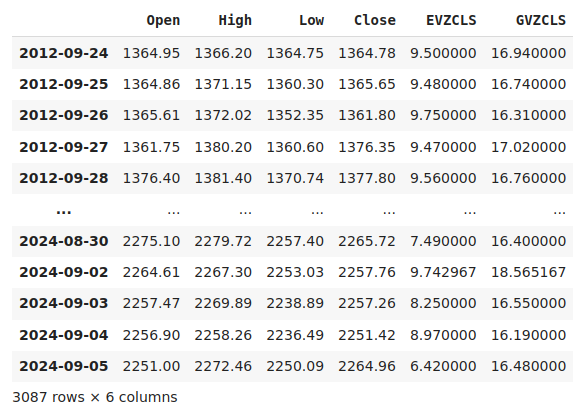
Fig 1: Our merged dataset
Labeling the data is an important step in any supervised machine learning project. First, we defined our forecast horizon, which in this case in 20 days into the future. Then, we defined the target as the future close price of the XAUEUR symbol. We also created binary targets to summarize whether price levels appreciated or depreciated. The binary targets will exclusively be used for visualization purposes.
#Let us label the data
look_ahead = 20

#Define the labels
merged_data["Target"] = merged_data["Close"].shift(-look_ahead)
merged_data["Binary Target"] = np.nan

merged_data.loc[merged_data["Target"] > merged_data["Close"],"Binary Target"] = 1
merged_data.loc[merged_data["Target"] <= merged_data["Close"],"Binary Target"] = 0

merged_data.dropna(inplace=True)
merged_data
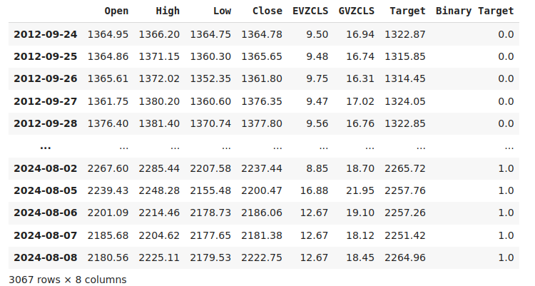
Fig 2: Our dataset with the target included
Finally, we defined the 3 set of predictors that we are going to empirically compare.
#Let us define the predictors and target
ohlc_predictors = ["Open","High","Low","Close"]
fred_predictors = ["EVZCLS","GVZCLS"]
predictors = ohlc_predictors + fred_predictors
target = "Target"
binary_target = "Binary Target"
Exploratory Data Analysis
The presence or absence of strong correlation levels does not necessarily imply the presence or absence of a relationship between data being analyzed. Our alternative data appears to have intermittent correlation levels with the XAUEUR dataset. However, there appeared to be strong correlation levels directly between the 2 alternative datasets.
#Exploratory Data Analysis
#Analyzing correlation levels
sns.heatmap(merged_data[predictors].corr(),annot=True)
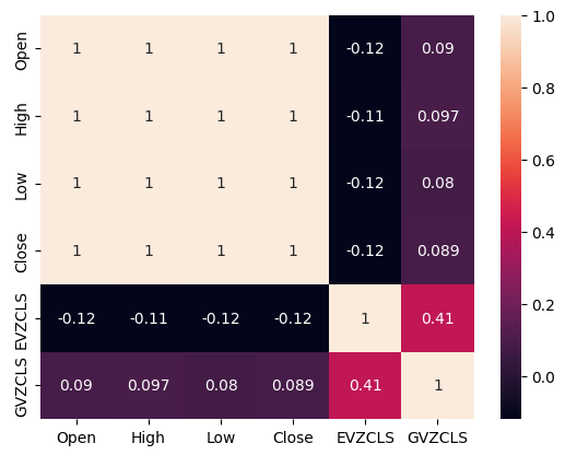
Fig 3: Our correlation heat map
We created 3 scatter plots of the data we have. The first 2 scatter plots used the Gold and Euro volatility index on the x-axis, and the XAUEUR close price on the y-axis in both plots. In our first scatter plot, it appears that when gold volatility levels rise above the 30-35 level, we consistently observed bullish price action.
#Let's create scatter plots
sns.scatterplot(data=merged_data,x="GVZCLS",y="Close",hue="Binary Target")
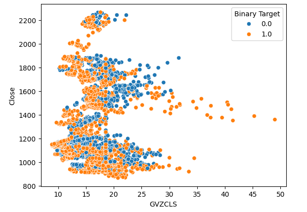
Fig 4: Our first scatter plot
The same phenomenon is observed in the second scatter plot. It appears that when Euro volatility levels rise beyond the 14-16 level, price levels consistently appreciated. However, our data set is limited and may not fully represent the true relationship between the 2 markets.
#Let's create scatter plots
sns.scatterplot(data=merged_data,x="EVZCLS",y="Close",hue="Binary Target")
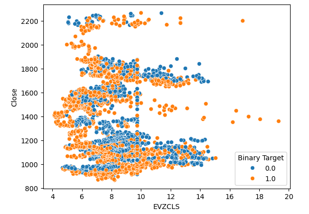
Fig 5: Our second scatter plot
Lastly, we created a scatter plot using our 2 alternative data sets on both axis. Our data created a cone like structure, with the cluster of bullish candles still clearly visible and well separated.
#Let's create scatter plots
sns.scatterplot(data=merged_data,x="GVZCLS",y="EVZCLS",hue="Binary Target")
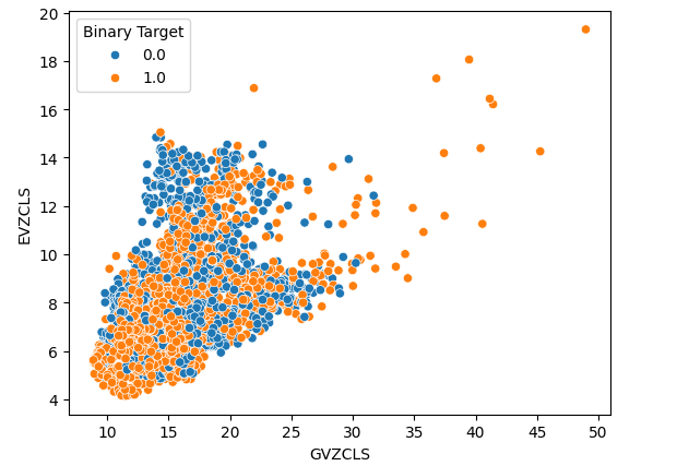
Fig 6: Our final scatter plot
There may be hidden structures in our data that cannot be visualized in 2 dimensions. Therefore, we created a 3D scatter plot to visualize the effect of both our alternative data sets on the XAUEUR. The cluster of bullish candles can still be clearly seen in the 3D plot. This may indicate that our alternative data is separating the data well at certain points.
#Define the 3D Plot
fig = plt.figure(figsize=(7,7))
ax = plt.axes(projection="3d")
ax.scatter(merged_data["GVZCLS"],merged_data["EVZCLS"],merged_data["Close"],c=merged_data["Binary Target"],cmap="plasma")
ax.set_xlabel("GVZCLS")
ax.set_ylabel("EVZCLS")
ax.set_zlabel("Close")
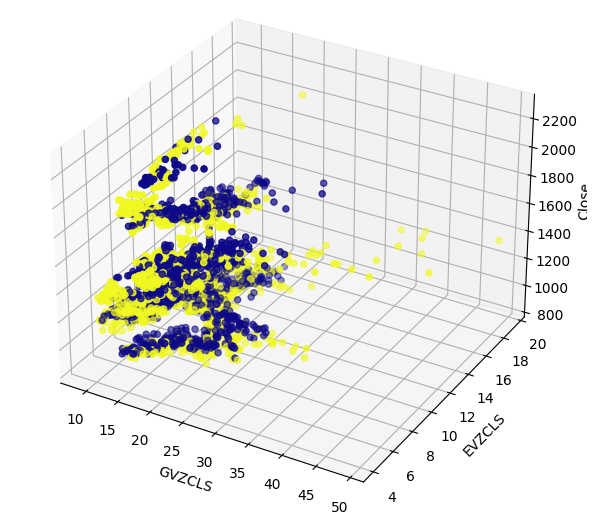
Fig 7: A 3D scatter plot of our market data
We can also employ dimensionality reduction techniques, to create a 2-dimensional representation of our 6-dimensional market data. We will use the t-SNE algorithm to accomplish this task. The algorithm was first proposed in a 2002 paper published by Geoffrey Hinton et al. The original paper can be found using this link, here. Hinton is considered a pioneer in the field of machine learning, largely for his 1986 paper demonstrating how the back-propagation algorithm can be used to train a neural network to predict the next word in a vector representation of a sentence. His contributions helped popularize the widespread adoption of the back-propagation algorithm.

Fig 8: Dr Geoffrey Hinton
The t-SNE algorithm is designed to create a compact representation of high dimensional data in which the proximity between all the data points in high dimensional space is preserved in the new lower dimensional representation. To achieve this goal, the algorithm minimizes a specialized cost function that measures the difference between two distributions. Normally, this optimization procedure is achieved by gradient descent. First, the algorithm creates a lower rank matrix of the original high dimensional data. Then, it iteratively moves the data points to minimize the cost, recall that the cost is the difference between the distributions of the data in the lower rank matrix and the original distribution of the data. The t-SNE algorithm is helpful for visualizing data clusters that are hidden in higher dimensional space.
We will import the libraries we need.
#Let's create a TSNE Plot
from sklearn.manifold import TS
Then we will instantiate the t-SNE object and instruct it to create a 2-dimensional representation of our data.
#Create a TSNE object which will reduce the data to 2 dimensions
tsne = TSNE(n_components=2,perplexity=30)
Fit the t-SNE object to the data we have.
#Apply TSNE to the data
tsne_data = tsne.fit_transform(merged_data[predictors])
Plotting the new representation of the data.
#Create a scatter plot
plt.scatter(tsne_data[:,0],tsne_data[:,1])
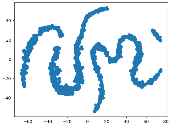
Fig 9: Our t-SNE plot of the market data
Due to the stochastic nature of the iterative optimization procedure, it may be challenging to reproduce the plot we have obtained in this discussion. Furthermore, if we performed the procedure a second time, we would not be alarmed if we obtained a different scatter plot. What we are particularly interested in, is the number of clusters the algorithm is trying to preserve. It appears our data set has 4 distinct clusters, furthermore the curved nature of the plots may suggest a dependency being shared across time within the clusters.
Autocorrelation (ACF) plots are used extensively in time-series analysis to inspect whether the data is stationary, contains seasonal fluctuations and a lot more. ACF plots show us the level of correlation between a time-series current value, and its previous values. We performed 3 ACF plots on the XAUEUR close and the 2 CBOE alternative data sets. All 3 plots, suggested that the data has persistent components, this was also suggested to us by the heat map we visualized earlier. When ACF plots have long tails that slowly decay to 0, we will naturally consider whether there could be strong trend or seasonal components in the data.
#Let's look at an autocorrelation plot of the data
close_acf = plot_acf(merged_data["Close"])
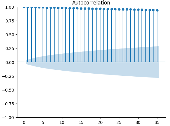
Fig 10: ACF plot of the XAUEUR Close price
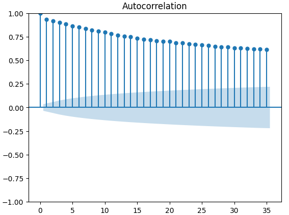
Fig 11: ACF plot of the CBOE Euro volatility index
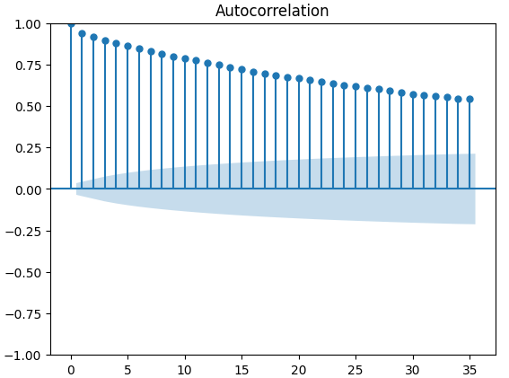
Fig 12: ACF plot of the CBOE Gold volatility index
Partial autocorrelation (PACF) plots inform us, how far back in time should we look to explain most of the correlation observed between the time-series and its lags. In other words, how much of the correlation observed in lag 3 was not being carried over from lag 2? All 3 of our PACF plots suggested to us that at most 4 lags account for most of the autocorrelation in the time-series data.
#Let's look at an partial autocorrelation plot of the close data
close_pacf = plot_pacf(merged_data["Close"])
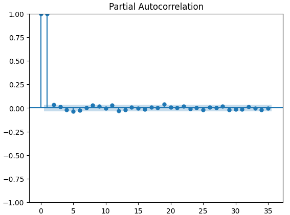
Fig 13: PACF plots of the XAUEUR close
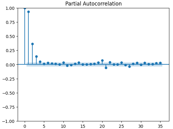
Fig 14: PACF plots of the CBOE Euro volatility index
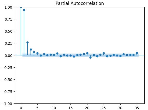
Fig 15: PACF plots of the CBOE Gold volatility index
Preparing To Model The Data
Before we can start modelling our data with our deep neural network, we must first make a few preparations.
#Preparing to model the data
from sklearn.preprocessing import RobustScaler
from sklearn.model_selection import TimeSeriesSplit,train_test_split
from sklearn.metrics import mean_squared_error
from sklearn.neural_network import MLPRegressor
The first step, is to standardize and scale the input data, so our model will learn effectively.
#Reset the index of our data
merged_data.reset_index(inplace=True)

X = merged_data.loc[:,predictors]
y = merged_data.loc[:,target]

#Scale our data
scaler = RobustScaler()
X = pd.DataFrame(scaler.fit_transform(merged_data[predictors]),columns=predictors)
Now we need to create train-test splits for the 3 set of predictors we have. Be careful not to randomly shuffle your data in this step. Otherwise, we would compromise the integrity of our analysis.
#Perform train test splits
ohlc_train_X,ohlc_test_X,train_y,test_y = train_test_split(X.loc[:,ohlc_predictors],y,shuffle=False,train_size=0.5)
fred_train_X,fred_test_X,_,_ = train_test_split(X.loc[:,fred_predictors],y,shuffle=False,train_size=0.5)
train_X,test_X,_,_ = train_test_split(X.loc[:,predictors],y,shuffle=False,train_size=0.5)
Lastly, we need to create our time series object and subsequently create a data frame to store our validation error levels.
#Let's now cross-validate each of the predictors
#Create the time-series split object
tscv = TimeSeriesSplit(n_splits=5,gap=look_ahead)

validation_error = pd.DataFrame(columns=["OHLC Predictors","FRED Predictors","All Predictors"],index=np.arange(0,5))
Modelling The Data
We are now ready to start modelling our data, and cross validating our models.
#Performing cross validation
model = MLPRegressor(hidden_layer_sizes=(20,5))
for i,(train,test) in enumerate(tscv.split(train_X)):
  model.fit(train_X.loc[train[0]:train[-1],:],train_y.loc[train[0]:train[-1]])
  validation_error.iloc[i,2] = mean_squared_error(train_y.loc[test[0]:test[-1]],model.predict(train_X.loc[test[0]:test[-1],:]))
Our validation error levels.
#Our validation error
validation_error | MetaTrader 5 OHLC Data | FRED CBOE Alternative Data | All The Data |
|---|---|---|
| 875423.637167 | 881892.498319 | 857846.11554 |
| 794999.120981 | 831138.370726 | 946193.178747 |
| 1058884.292095 | 474744.732539 | 631259.842972 |
| 419566.842693 | 882615.372658 | 483408.373559 |
| 96693.318078 | 618647.934237 | 237935.04009 |
It may not be immediately obvious to us which model is performing best, however when we analyze the column means, we can clearly see the last model is performing exceptionally. In the plot below, we subtracted the mean value of the first column, from the remaining columns. By doing so, the first column value is 0 and all unsatisfactory models will have column values greater than 0. Therefore, we can clearly see that our last model is performing quite well.
#Our mean error levels
val_err = validation_error.mean()
val_err = val_err.iloc[:] - val_err.iloc[0]
val_err.plot(kind="bar")
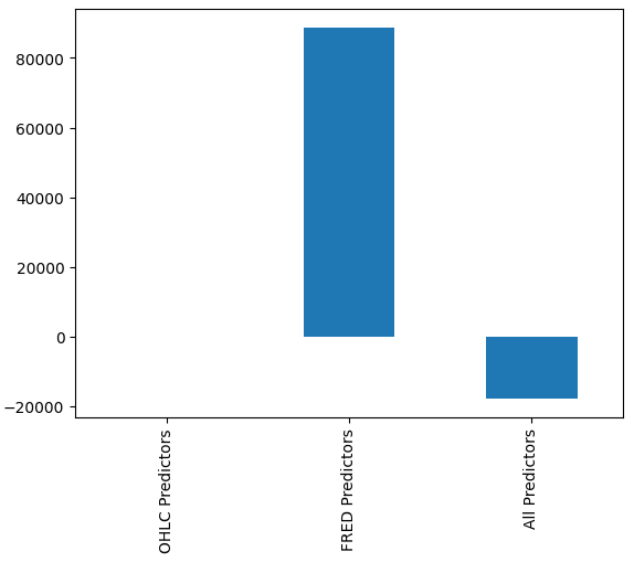
Fig 16: Our model's performance using 3 different data sets
Performing box plots of the model’s performance further shows that the last set of predictors appear to be the optimal choice for us, the mean error rate is the lowest, and the variance is not as large as it is when just using OHCL data.
#Let's perform boxplots of our validation error
sns.boxplot(validation_error)
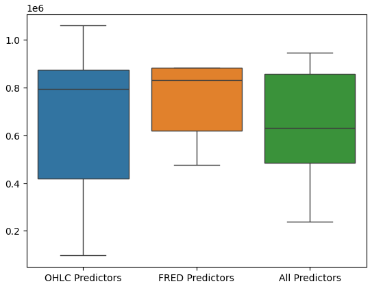
Fig 17: Our model's performance visualized as box plots
Feature Importance
We should never blindly trust any model and deploy it into production simply because it produced low error metrics. Let us inspect the relationships the model has learned. We would like to gain an understanding of global feature importance to our model. We will start off by creating Accumulated Local Effect (ALE) plots. ALE is designed to provide robust explanations for machine learning models that are trained on data with high levels of correlation. ALE attempts to isolate the effect each input has on the model’s output.
#Feature importance
from alibi.explainers import ALE , plot_ale
We will now instantiate our ALE object and fetch explanations on global feature importance for our deep neural network. This will help us understand the effect each of our inputs appears to have on the model prediction.
#Explaining our deep neural network
model = MLPRegressor(hidden_layer_sizes=(20,5))
model.fit(train_X,train_y)
dnn_ale = ALE(model.predict,feature_names=predictors,target_names=["XAUEUR Close"])
Let us now calculate and plot our ALE values for each of the model’s inputs.
#Obtaining the explanation
ale_X = X.to_numpy()
dnn_explanations = dnn_ale.explain(ale_X)
#Plotting feature importance
plot_ale(dnn_explanations,n_cols=3,fig_kw={'figwidth':8,'figheight':8},sharey=None) 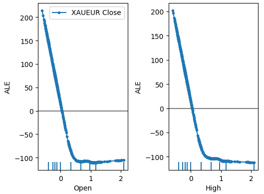
Fig 18: Our ALE plots for some of the XAUEUR Open and High predictors
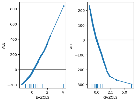
Fig 19: Our ALE plots for the FRED CBOE volatility indexes
Interpreting ALE plots is quite intuitive, the plot illustrates how the model’s prediction changes as the value of each predictor changes. As we can see, as the Open and High price increase, the model’s prediction initially falls. However, it becomes less sensitive as the price levels continue increasing. Although we didn’t include them here, the ALE plots of the Low and Close price look identical to the 2 plots we showed.
When we now turn our attention to the ALE plots of the alternative data, we observe that the Euro volatility index created an ALE plot that covers part of the graph that the other variables failed to cover. In other words, the predictor appears to be explaining variance in the target that we were unable to explain without it. Furthermore, the upward slope of the ALE plot suggest that as the predictor’s value increases, so does the model’s forecast.
Next we will retrieve SHAP explanations for our model’s performance. SHAP values help us quantify how each of the model’s inputs contributed to a specific prediction when compared to the model’s average prediction. SHAP values are rooted in the mathematical field of game theory. The algorithm considered each possible set of predictors, and then calculates the average effect of the inputs across all possible sets.
First, we will import the SHAP library.
#SHAP Values
import shap
Calculate the SHAP values.
#Calculating SHAP values
explainer = shap.Explainer(model.predict,train_X)
shap_values = explainer(test_X)#Calculating SHAP values
Plot the SHAP values.
#Plot the beeswarm plot
shap.plots.beeswarm(shap_values) 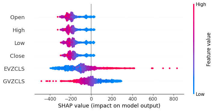
Fig 20: Our SHAP explanations
According to our SHAP explanations, the market data fetched from the XAUEUR market itself, is the most important data we have. Furthermore, the SHAP plot also suggests to us that as the current market price increases, the target tends to fall.
Parameter Tuning
Let us try to gain more performance from our model, we will start by importing the libraries we need.
#Parameter tuning
from sklearn.model_selection import RandomizedSearchCV
Initialize the model.
#Reinitialize the model
model = MLPRegressor(hidden_layer_sizes=(20,5))
Define the tuner object.
#Define the tuner
tuner = RandomizedSearchCV(
        model,
        {
        "activation" : ["relu","logistic","tanh","identity"],
        "solver":["adam","sgd","lbfgs"],
        "alpha":[0.1,0.01,0.001,0.0001,0.00001,0.00001,0.0000001],
        "tol":[0.1,0.01,0.001,0.0001,0.00001,0.000001,0.0000001],
        "learning_rate":['constant','adaptive','invscaling'],
        "shuffle": [True,False]
        },
        n_iter=500,
        cv=5,
        n_jobs=-1,
        scoring="neg_mean_squared_error"
)
Fit the tuner.
#Fit the tuner
tuner_results = tuner.fit(train_X,train_y)
The best parameters we found.
#The best parameters we found
tuner_results.best_params_ 'solver': 'lbfgs',
'shuffle': True,
'learning_rate': 'adaptive',
'alpha': 0.1,
'activation': 'identity'}
Scipy has optimization procedures included in its minimize module. These procedures require a starting point for the optimization process. We will use the best parameter values found by random search as the starting point in our second optimization phase.
#Deeper optimization
from scipy.optimize import minimize
Now, we will create a data frame object to store our error levels in validation.
#Create a dataframe to store our accuracy
current_error_rate = pd.DataFrame(index = np.arange(0,5),columns=["Current Error"])
Every optimization algorithm needs an objective function to work on. In our case, the objective function is average cross validated error of the model on the training set. Our optimization procedure will look for model parameters that minimize our average error.
#Define the objective function
def objective(x):
    #The parameter x represents a new value for our neural network's settings
    #In order to find optimal settings, we will perform 10 fold cross validation using the new setting
    #And return the average RMSE from all 10 tests
    #We will first turn the model's Alpha parameter, which controls the amount of L2 regularization
    model = MLPRegressor(hidden_layer_sizes=(20,5),activation='identity',learning_rate='adaptive',solver='lbfgs',shuffle=True,alpha=x[0],tol=x[1])
    #Now we will cross validate the model
    for i,(train,test) in enumerate(tscv.split(train_X)):
        #Train the model
        model.fit(train_X.loc[train[0]:train[-1],:],train_y.loc[train[0]:train[-1]])
        #Measure the RMSE
        current_error_rate.iloc[i,0] = mean_squared_error(train_y.loc[test[0]:test[-1]],model.predict(train_X.loc[test[0]:test[-1],:]))
    #Return the Mean CV RMSE
    return(current_error_rate.iloc[:,0].mean())
Let us define the starting point for the optimization procedure, and we should also define bounds for allowed input values.
#Define the starting point
pt = [0.1,0.00000001]
bnds = ((0.0000000000000000001,10000000000),(0.0000000000000000001,10000000000))
Optimizing the model.
#Searchin deeper for parameters
result = minimize(objective,pt,method="L-BFGS-B",bounds=bnds)
Testing For Overfitting
Overfitting is a problem in any machine learning project. It occurs when our model fails to create meaningful generalizations of the data, and rather begins to learn noise and other meaningless associations in the data. To test for overfitting, we will compare the accuracy of our 2 customized models, against the default model.
#Testing for overfitting
default_model          = MLPRegressor(hidden_layer_sizes=(20,5))
customized_model       = MLPRegressor(hidden_layer_sizes=(20,5),activation='identity',learning_rate='adaptive',solver='lbfgs',shuffle=True,alpha=0.1,tol=0.0000001)
customized_lbfgs_model = MLPRegressor(hidden_layer_sizes=(20,5),activation='identity',learning_rate='adaptive',solver='lbfgs',shuffle=True,alpha=result.x[0],tol=result.x[1])
Let us now prepare to cross-validate each model.
#Preparing to cross validate the models
models = [
    default_model,
    customized_model,
    customized_lbfgs_model
]

#We will store our validation error here
validation_error = pd.DataFrame(columns=["Default Model","Customized Model","L-BFGS Model"],index=np.arange(0,5))

#We will now reset the indexes
test_y = test_y.reset_index()
test_X = test_X.reset_index()
We should fit each of the models on the training set.
#Fit each of the models
for m in models:
  m.fit(train_X,train_y)
Now, let us cross-validate our model's performance on unseen data, the test set that we have held out until now.
#Cross validating each model
for j in np.arange(0,len(models)):
  model = models[j]
  for i,(train,test) in enumerate(tscv.split(test_X)):
    model.fit(test_X.loc[train[0]:train[-1],:],test_y.loc[train[0]:train[-1],"Target"])
    validation_error.iloc[i,j] = mean_squared_error(test_y.loc[test[0]:test[-1],"Target"],model.predict(test_X.loc[test[0]:test[-1],:]))
Our validation error levels.
#Our validation error
validation_error | Default Model | Randomized Search Model | L-BFGS-B Model |
|---|---|---|
| 22360.060721 | 5917.062055 | 3734.212826 |
| 17385.289026 | 36726.684574 | 35886.972729 |
| 13782.649037 | 5128.022626 | 20886.845316 |
| 3082484.290698 | 6950.786438 | 5789.948045 |
| 4076009.132941 | 27729.589769 | 22931.572161 |
The best performing model is the Randomized search model.
#Plotting the difference in our performance levels
mean = validation_error.mean()
mean = mean.iloc[:] - mean.iloc[0]
mean.plot(kind="bar")
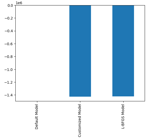
Fig 21: Our validation error levels
Visualizing our model's performance makes it clear how poorly the default model is handling the data.
#Visualizing the results
validation_error.plot() 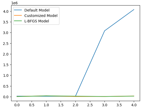
Fig 22: Testing for overfitting
This point is reinforced further by our box plots. We can tell that we have surpassed the default model by a considerable margin.
#Visualizing our results
sns.boxplot(validation_error) 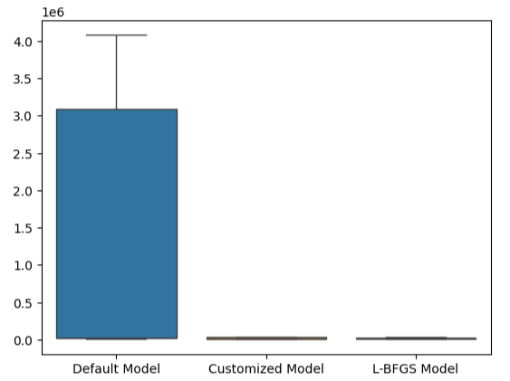
Fig 23: We are outperforming the default model by a wide margin
Preparing To Export To ONNX Format
Before we can export our model to ONNX format, we must first standardize and scale our data in a fashion that we can reproduce in our MetaTrader 5 Terminal. To achieve this, we will subtract the column mean from each column, before we finally divide each column by its standard deviation. We will write out our scaling factors in CSV format so that we can retrieve them in our MetaTrader 5 terminal to scale our model inputs.
#Let us now prepare to export our model to onnx format
scale_factors = pd.DataFrame(columns=predictors,index=["mean","standard deviation"])

for i in np.arange(0,len(predictors)):
  scale_factors.iloc[0,i] = merged_data.loc[:,predictors[i]].mean()
  scale_factors.iloc[1,i] =  merged_data.loc[:,predictors[i]].std()
  merged_data.loc[:,predictors[i]] = (merged_data.loc[:,predictors[i]] - merged_data.loc[:,predictors[i]].mean())/merged_data.loc[:,predictors[i]].std()

scale_factors
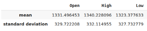
Fig 24: Some of our scaling factors
Now we will write out the data in CSV format.
#Save the scale factors to CSV
scale_factors.to_csv("scale_factors.csv")
Exporting To ONNX Format
Open Neural Network Exchange (ONNX) is a protocol for building and sharing machine learning models across different programming languages. The ONNX protocol allows us to seamlessly embed our deep neural network into our Expert Advisor using the MQL5 ONNX API.
Let us first load the libraries we need.
#Exporting to ONNX format
import onnx
from skl2onnx import convert_sklearn
from skl2onnx.common.data_types import FloatTensorType
Train the model on all the data we have.
#Fit the model on all the data we have
customized_model.fit(merged_data.loc[:,predictors],merged_data.loc[:,target])
When exporting ONNX models, the input shape may be lost. Therefore, let us explicitly specify the input shape.
# Define the input type
initial_types = [("float_input",FloatTensorType([1,6]))]
Create the ONNX representation of the model.
# Create the ONNX representation
onnx_model = convert_sklearn(customized_model,initial_types=initial_types,target_opset=12)
Save the ONNX representation to a file with the ".onnx" extension.
# Save the ONNX model
onnx_name = "XAUEUR FRED D1.onnx"
onnx.save_model(onnx_model,onnx_name)
Getting Up-To-Date FRED Data
Before we can start building our Expert Advisor, we need to create a Python script that will constantly share up-to-date FRED data with our Terminal. We will create a script that will fetch the latest data available once a day and write it out in CSV in the "Files" folder so that we can access the data with our trading application.
#A function to write out our alternative data to CSV
def write_out_alternative_data():
        euro = fred.get_series("EVZCLS")
        euro = euro.iloc[-1]
        gold = fred.get_series("GVZCLS")
        gold = gold.iloc[-1]
        data = pd.DataFrame(np.array([euro,gold]),columns=["Data"],index=["Fred Euro","Fred Gold"])
        data.to_csv("C:\\ENTER\\YOUR\\PATH\\HERE\\MetaQuotes\\Terminal\\D0E8209F77C8CF37AD8BF550E51FF075\\MQL5\\Files\\fred_xau_eur.csv")
Now we will write out an infinite loop, to write out the data and then sleep for one day.
while True:
        #Update the fred data for our MT5 EA
        write_out_alternative_data()
        #If we have finished all checks then we can wait for one day before checking for new data
        time.sleep(24 * 60 * 60)
Building Our Expert Advisor
We are now prepared to start building our Expert Advisor. We will start off by first requiring the ONNX file we have just created.
//+------------------------------------------------------------------+
//|                                               EURXAU Fred AI.mq5 |
//|                                        Gamuchirai Zororo Ndawana |
//|                          https://www.mql5.com/en/gamuchiraindawa |
//+------------------------------------------------------------------+
#property copyright "Volatility Doctor"
#property link      "https://www.mql5.com/en/gamuchiraindawa"
#property version   "1.00"

//+------------------------------------------------------------------+
//| Require the ONNX file                                            |
//+------------------------------------------------------------------+
#resource "\\Files\\XAUEUR FRED D1.onnx" as const uchar onnx_buffer[];
Load the trade library to help us manage our positions.
//+------------------------------------------------------------------+
//| Libraries                                                        |
//+------------------------------------------------------------------+
#include  <Trade/Trade.mqh>
CTrade Trade;
These global variables will be shared in many different parts of our application.
//+------------------------------------------------------------------+
//| Global variables                                                 |
//+------------------------------------------------------------------+
long    onnx_model;
vector  mean_values  = vector::Zeros(6);
vector  std_values   = vector::Zeros(6);
vectorf model_inputs = vectorf::Zeros(6);
vectorf model_output = vectorf::Zeros(1);
double  bid,ask;
int     system_state,model_sate;
Now, we need a function that will create our ONNX model, from the ONNX buffer we created at the beginning of our application. Our function will first create and validate the ONNX model, and lastly it will set and validate the model's input and output shapes. If we fail at any point, the function will return false, which in turn will halt the initialization procedure.
//+------------------------------------------------------------------+
//| Load the ONNX file                                               |
//+------------------------------------------------------------------+
bool load_onnx_file(void)
  {
//--- Create the ONNX model from the buffer we loaded earlier
   onnx_model = OnnxCreateFromBuffer(onnx_buffer,ONNX_DEFAULT);

//--- Validate the model we just created
   if(onnx_model == INVALID_HANDLE)
     {
      //--- Give the user feedback on the error
      Comment("Failed to create the ONNX model: ",GetLastError());
      //--- Break initialization
      return(false);
     }

//--- Define the I/O shape
   ulong input_shape [] = {1,6};

//--- Validate the input shape
   if(!OnnxSetInputShape(onnx_model,0,input_shape))
     {
      //--- Give the user feedback
      Comment("Failed to define the ONNX input shape: ",GetLastError());
      //--- Break initialization
      return(false);
     }

   ulong output_shape [] = {1,1};

//--- Validate the output shape
   if(!OnnxSetOutputShape(onnx_model,0,output_shape))
     {
      //--- Give the user feedback
      Comment("Failed to define the ONNX output shape: ",GetLastError());
      //--- Break initialization
      return(false);
     }

//--- We've finished
   return(true);
  }
//+------------------------------------------------------------------+
From there, we will now define the scaling factors we will need to normalize our model inputs.
//+------------------------------------------------------------------+
//| Load our scaling factors                                         |
//+------------------------------------------------------------------+
bool load_scaling_factors(void)
  {
//--- Load the scaling values
   mean_values[0] = 1331.4964525595044;
   mean_values[1] = 1340.2280958591457;
   mean_values[2] = 1323.3776328659928;
   mean_values[3] = 1331.706768829475;
   mean_values[4] = 8.258127607767035;
   mean_values[5] = 16.35582438284101;
   std_values[0] = 329.7222075527991;
   std_values[1] = 332.11495530642173;
   std_values[2] = 327.732778866831;
   std_values[3] = 330.1146052811378;
   std_values[4] = 2.199782202942867;
   std_values[5] = 4.241112965400358;

//--- Validate the values loaded correctly
   if((mean_values.Sum() > 0) && (std_values.Sum() > 0))
     {
      return(true);
     }

//--- We failed to load the scaling values
   return(false);
  }
Whenever our application is no longer in use, we will free up the resources we are no longer using.
//+------------------------------------------------------------------+
//| Free up the resources we no longer need                          |
//+------------------------------------------------------------------+
void release_resources(void)
  {
//--- Free up all the resources we have used so far
   OnnxRelease(onnx_model);
   ExpertRemove();
   Print("Thank you for choosing Volatility Doctor");
  }
This function will be responsible for updating our market price information.
//+------------------------------------------------------------------+
//| Fetch market data                                                |
//+------------------------------------------------------------------+
void fetch_market_data(void)
  {
//--- Update the market data
   bid = SymbolInfoDouble(Symbol(),SYMBOL_BID);
   ask = SymbolInfoDouble(Symbol(),SYMBOL_ASK);
  }
The following function is responsible for fetching a prediction from our model. First, we will fetch the current OHLC data on the XAUEUR symbol using the MQL5 matrix function CopyRates(). After fetching the data, we will normalize it and store it in the input vector we defined earlier. From here, we will call another function to read the latest FRED data we have on file.
//+------------------------------------------------------------------+
//| This function will fetch a prediction from our model             |
//+------------------------------------------------------------------+
void model_predict(void)
  {
//--- Get the input data ready
   for(int i =0; i < 6; i++)
     {
      //--- The first 4 inputs will be fetched from the market
      matrix xau_eur_ohlc = matrix::Zeros(1,4);
      xau_eur_ohlc.CopyRates(Symbol(),PERIOD_D1,COPY_RATES_OHLC,0,1);
      //--- Fill in the data
      if(i<4)
        {
         model_inputs[i] = (float)((xau_eur_ohlc[i,0] - mean_values[i])/ std_values[i]);
        }
      //--- We have to read in the fred alternative data
      else
        {
         read_fred_data();
        }
     }
  }
The function, defined below, will read in the CSV file with the latest FRED data and normalize the data before storing it in the input vector and fetching a prediction from our model. We will represent the model's prediction using an integer. This will help us quickly spot potential reversals and close our positions, hopefully on the right side of the market.
//+-------------------------------------------------------------------+
//| Read in the FRED data                                             |
//+-------------------------------------------------------------------+
void read_fred_data(void)
  {
//--- Read in the file
   string file_name = "fred_xau_eur.csv";

//--- Try open the file
   int result = FileOpen(file_name,FILE_READ|FILE_CSV|FILE_ANSI,","); //Strings of ANSI type (one byte symbols).

//--- Check the result
   if(result != INVALID_HANDLE)
     {
      Print("Opened the file");
      //--- Store the values of the file

      int counter = 0;
      string value = "";
      while(!FileIsEnding(result) && !IsStopped()) //read the entire csv file to the end
        {
         if(counter > 10)  //if you aim to read 10 values set a break point after 10 elements have been read
            break;          //stop the reading progress

         value = FileReadString(result);
         Print("Counter: ");
         Print(counter);
         Print("Trying to read string: ",value);

         if(counter == 3)
           {
            Print("Fred Euro data: ",value);
            model_inputs[4] = (float)((((float) value) - mean_values[4])/std_values[4]);
           }

         if(counter == 5)
           {
            Print("Fred Gold data: ",value);
            model_inputs[5] = (float)((((float) value) - mean_values[5])/std_values[5]);
           }

         if(FileIsLineEnding(result))
           {
            Print("row++");
           }

         counter++;
        }

      //--- Show the input and Fred data
      Print("Input Data: ");
      Print(model_inputs);

      //---Close the file
      FileClose(result);

      //--- Store the model prediction
      OnnxRun(onnx_model,ONNX_DEFAULT,model_inputs,model_output);
      Comment("Model Forecast",model_output[0]);
      if(model_output[0] > iClose(Symbol(),PERIOD_D1,0))
        {
         model_sate = 1;
        }

      else
        {
         model_sate = -1;
        }
     }

//--- We failed to find the file
   else
     {
      //--- Give the user feedback
      Print("We failed to find the file with the FRED data");
     }
  }
Let us now define how our application should start up. Our application should first create the ONNX model and then load the scaling factors we need. If either one of these steps should fail, we will abort the initialization procedure altogether.
//+------------------------------------------------------------------+
//| Expert initialization function                                   |
//+------------------------------------------------------------------+
int OnInit()
  {
//--- Load the ONNX model
   if(!load_onnx_file())
     {
      //--- We failed to load our ONNX model
      return(INIT_FAILED);
     }

//--- Load the scaling factors
   if(!load_scaling_factors())
     {
      //--- We failed to read in the scaling factors
      return(INIT_FAILED);
     }

//--- We mamnaged to load our model
   return(INIT_SUCCEEDED);
  }
When our application has been removed from the chart, release the resources we no longer need.
//+------------------------------------------------------------------+
//| Expert deinitialization function                                 |
//+------------------------------------------------------------------+
void OnDeinit(const int reason)
  {
//--- Free up the resources we no longer need
   release_resources();
  }
Finally, whenever we receive updated market quotes, we will first store the updated market prices in memory. Subsequently, if we have no open positions, we will follow our model's prediction only if it is supported by price action on higher time frames. Alternatively, if we already have open positions, we will close our positions if our model is anticipating reversals in price levels.
//+------------------------------------------------------------------+
//| Expert tick function                                             |
//+------------------------------------------------------------------+
void OnTick()
  {
//--- Update market data
   fetch_market_data();

//--- Fetch a prediction from our model
   model_predict();

//--- If we have no positions follow the model's lead
   if(PositionsTotal() == 0)
     {
      //--- Buy position
      if(model_sate == 1)
        {
         if(iClose(Symbol(),PERIOD_W1,0) > iClose(Symbol(),PERIOD_W1,12))
           {
            Trade.Buy(0.3,Symbol(),ask,0,0,"XAUEUR Fred AI");
            system_state = 1;
           }
        };

      //--- Sell position
      if(model_sate == -1)
        {
         if(iClose(Symbol(),PERIOD_W1,0) < iClose(Symbol(),PERIOD_W1,12))
           {
            Trade.Sell(0.3,Symbol(),bid,0,0,"XAUEUR Fred AI");
            system_state = -1;
           }
        };
     }

//--- If we allready have positions open, let's manage them
   if(model_sate != system_state)
     {
      Trade.PositionClose(Symbol());
     }

  }
//+------------------------------------------------------------------+

Fig 25: Our Expert Advisor in action
Conclusion
In this article, we have demonstrated that there may be virtue in including the FRED CBOE Volatility Indexes to help improve the accuracy of your machine learning models. While we cannot guarantee that the information provided in this article will consistently generate success, it is certainly worth considering if you are ready to start employing alternative data into your trading strategies.
- Free trading apps
- Over 8,000 signals for copying
- Economic news for exploring financial markets
You agree to website policy and terms of use