Reimagining Classic Strategies in MQL5 (Part III): FTSE 100 Forecasting

MetaTrader 5 — Examples | 23 September 2024, 14:20

2 156

Artificial Intelligence (AI) yields potentially infinite use cases in the strategy of the modern investor. Regrettably, no single investor may have enough time to carefully analyze each strategy before deciding which one to trust with their capital. In this series of articles, we will help you traverse the vast landscape of possible AI-based strategies, to help you identify a strategy that suits your investor profile.

Trading Strategy Overview

The London Stock Exchange (LSE) is one of the oldest stock exchanges in the developed world. It was founded in 1801, and is the primary stock exchange of the United Kingdom. It is considered part of the big 3 alongside the New York Stock Exchange and the Tokyo Stock Exchange. The London Stock Exchange is the largest stock exchange in Europe and according to their Official website, the current total market capitalization of all companies listed on the exchange is approximately 4.4 trillion British Pounds.

The Financial Times Stock Exchange (FTSE) 100, is an index derived from the LSE that tracks the 100 largest companies listed on the LSE. These companies are commonly referred to as blue-chip stocks, and they are seen as relatively safe investments given the reputation earned by the companies over time and their proven track record. We can take advantage of our understanding of how the FTSE 100 Index is calculated, and potentially create a new trading strategy that will forecast the future closing price of the FTSE 100, by considering the current close price of the index, as well as the performance of 10 large stocks listed in the index.

Methodology Overview

We built our AI-powered Expert Advisor completely in MQL5. This gives us flexibility because our model can be used on different time frames without having to be constantly adjusted. Furthermore, we can dynamically adjust model parameters, such as how far into the future the model should forecast. Our model used 12 inputs in total to forecast the future close price of the FTSE 100, 20 steps into the future.

We performed Z-standardization to normalize and scale each of our model inputs using the column mean and standard deviation values. Our target was the future close price of the FTSE100 Index 20 steps into the future, and we created a multiple Linear Regression model to forecast the future close price of the index.

Not all machine learning models are created equally, this is especially evident in tasks that concern forecasting. Let us consider decision trees, tree algorithms generally work by partitioning the data into groups and then whenever the model is required to make a prediction, it simply returns the group mean for whichever group best matches the current input data. Therefore, tree-based algorithms do not perform extrapolation, in other words they do not possess the skill to look forward and make a prediction into the future. Therefore, if a tree-based model were given 5 similar inputs from 5 different moments, it could forecast the same closing price for all 5 if they were similar enough, whereas our linear regression model is capable of extrapolation, and can give us a forecast about the future close price of a security.

Initial Design As A Script

We will initially build our idea as a simple script in MQL5 so we can appreciate how the pieces of our system work together. We will start off by defining our global variables.

//+------------------------------------------------------------------+
//|                                                        UK100.mq5 |
//|                                        Gamuchirai Zororo Ndawana |
//|                          https://www.mql5.com/en/gamuchiraindawa |
//+------------------------------------------------------------------+
#property copyright "Gamuchirai Zororo Ndawana"
#property link      "https://www.mql5.com/en/gamuchiraindawa"
#property version   "1.00"
//+------------------------------------------------------------------+
//| Script program start function                                    |
//+------------------------------------------------------------------+

//1) ADM.LSE  - Admiral
//2) AAL.LSE  - Anglo American
//3) ANTO.LSE - Antofagasta
//4) AHT.LSE  - Ashtead
//5) AZN.LSE  - AstraZeneca
//6) ABF.LSE  - Associated British Foods
//7) AV.LSE   - Aviva
//8) BARC.LSE - Barclays
//9) BP.LSE   - BP
//10) BKG.LSE - Berkeley Group 
//11) UK100   - FTSE 100 Index

//+-------------------------------------------------------------------+
//| Global variables                                                  |
//+-------------------------------------------------------------------+
int fetch = 2000;
int look_ahead = 20;
double mean_values[11],std_values[11];
string list_of_companies[11] = {"ADM.LSE","AAL.LSE","ANTO.LSE","AHT.LSE","AZN.LSE","ABF.LSE","AV.LSE","BARC.LSE","BP.LSE","BKG.LSE","UK100"};
vector intercept = vector::Ones(fetch);
matrix target = matrix::Zeros(1,fetch);
matrix coefficients;
matrix input_matrix = matrix::Zeros(12,fetch);

The first task we will complete is fetching and normalizing the input data. We will store the input data in one matrix, and the target data will be kept in its own matrix

void OnStart()
  {
//--- Fetch the target
target.CopyRates("UK100",PERIOD_CURRENT,COPY_RATES_CLOSE,1,fetch);

//--- Fill in the input matrix
for(int i = 0; i < 11; i++)
   {
      //--- Add the symbol to market watch
      SymbolSelect(list_of_companies[i],true);
      //--- Fetch historical data
      vector temp = vector::Zeros(fetch);
      temp.CopyRates(list_of_companies[i],PERIOD_CURRENT,COPY_RATES_CLOSE,1+look_ahead,fetch);
      //--- Store the mean value and standard deviation, also scale the data
      mean_values[i] = temp.Mean();
      std_values[i] = temp.Std();
      temp = ((temp - mean_values[i]) / std_values[i]);
      //--- Add the data to the matrix
      input_matrix.Row(temp,i);
   }
//--- Add the intercept
input_matrix.Row(intercept,11);

//--- Show the input data
Print("Input data:");
Print(input_matrix);

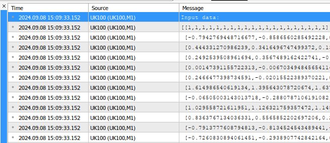
Fig 1: An example of the output generated by our script

After fetching our input data, we can now proceed to calculate our model parameters. Fortunately, the coefficients of a multiple linear regression model can be calculated by a closed form formula. We can observe an example of the model coefficients below.

//--- Calculating coefficient values
coefficients = target.MatMul(input_matrix.PInv());

//--- Display the coefficient values
Print("UK100 Coefficients:");
Print(coefficients.Transpose());

UK100 Coefficients

Fig 2: Our model parameters

Let us interpret the results together, the first coefficient value represent the average value of the target when all model inputs are 0. This is the mathematical definition of the bias parameter. However, in our trading application, it makes very little intuitive sense. Technically speaking, if all the stocks in the FTSE 100 were valued at 0 British Pounds, then the average future value of the FTSE 100 would also be 0 British Pounds. The second coefficient term, represents the marginal change in the future value of the FTSE 100, assuming all other stocks close at the same price. Therefore, whenever Admiral stocks increase by one unit, we observe that the future close price of the index appears to fall, slightly.

Obtaining a prediction from our model is as simple as multiplying the current price of each stock, by its calculated coefficient value, and summing all these products. Now that we have an idea of how we can build our model, we are ready to start building our Expert Advisor.

Implementing Our Expert Advisor

We will start off by defining inputs the user can change, to alter the behavior of the program.

//+------------------------------------------------------------------+
//|                                                  FTSE 100 AI.mq5 |
//|                                        Gamuchirai Zororo Ndawana |
//|                          https://www.mql5.com/en/gamuchiraindawa |
//+------------------------------------------------------------------+
#property copyright "Gamuchirai Zororo Ndawana"
#property link      "https://www.mql5.com/en/gamuchiraindawa"
#property version   "1.00"

//+------------------------------------------------------------------+
//| User inputs                                                      |
//+------------------------------------------------------------------+
input int look_ahead = 20;       // How far into the future should we forecast?
input int rsi_period = 20;       // The period of our RSI
input int profit_target = 20;     // After how much profit should we close our positions?
input bool ai_auto_close = true; // Should the AI automatically close positions?

Then we will import the trade library to help us manage our positions.

//+------------------------------------------------------------------+
//| Libraries we need                                                |
//+------------------------------------------------------------------+
#include  <Trade/Trade.mqh>
CTrade Trade;

Now we shall define a few global variables that we will need throughout our Expert Advisor.

//+------------------------------------------------------------------+
//| Global variables                                                 |
//+------------------------------------------------------------------+
double position_profit = 0;
int fetch = 20;
matrix coefficients;
matrix input_matrix = matrix::Zeros(12,fetch);
double mean_values[11],std_values[11],rsi_buffer[1];
string list_of_companies[11] = {"ADM.LSE","AAL.LSE","ANTO.LSE","AHT.LSE","AZN.LSE","ABF.LSE","AV.LSE","BARC.LSE","BP.LSE","BKG.LSE","UK100"};
ulong open_ticket;

We shall now define a function for fetching our training data. Recall that we aim to fetch the training data, and then normalize and standardize our data before adding it to the input matrix.

//+------------------------------------------------------------------+
//| This function will fetch our training data                       |
//+------------------------------------------------------------------+
void fetch_training_data(void)
  {
//--- Fetch the target
   target.CopyRates("UK100",PERIOD_CURRENT,COPY_RATES_CLOSE,1,fetch);

//--- Add the intercept
   input_matrix.Row(intercept,0);

//--- Fill in the input matrix
   for(int i = 0; i < 11; i++)
     {
      //--- Add the symbol to market watch
      SymbolSelect(list_of_companies[i],true);
      //--- Fetch historical data
      vector temp = vector::Zeros(fetch);
      temp.CopyRates(list_of_companies[i],PERIOD_CURRENT,COPY_RATES_CLOSE,1+look_ahead,fetch);
      //--- Store the mean value and standard deviation, also scale the data
      mean_values[i] = temp.Mean();
      std_values[i] = temp.Std();
      temp = ((temp - mean_values[i]) / std_values[i]);
      //--- Add the data to the matrix
      input_matrix.Row(temp,i+1);
     }
  }

After fetching our training data, we should also define a function for fitting our model coefficients.

//+---------------------------------------------------------------------+
//| This function will fit our multiple linear regression model         |
//+---------------------------------------------------------------------+
void model_fit(void)
  {
//--- Calculating coefficient values
   coefficients = target.MatMul(input_matrix.PInv());
  }

Once we have trained and fitted our model, we can finally get predictions from our model. We will first fetch and normalize current market data from our model to get started. After fetching the data, we apply the linear regression formula to obtain a forecast from our model. Then, finally, we will store the model’s forecast as a binary flag to help us keep track of potential reversals.

//+---------------------------------------------------------------------+
//| This function will fetch a prediction from our model                |
//+---------------------------------------------------------------------+
void model_predict(void)
  {
//--- Add the intercept
   intercept = vector::Ones(1);
   input_matrix.Row(intercept,0);

//--- Fill in the input matrix
   for(int i = 0; i < 11; i++)
     {
      //--- Fetch historical data
      vector temp = vector::Zeros(1);
      temp.CopyRates(list_of_companies[i],PERIOD_CURRENT,COPY_RATES_CLOSE,0,1);
      //--- Normalize and scale the data
      temp = ((temp - mean_values[i]) / std_values[i]);
      //--- Add the data to the matrix
      input_matrix.Row(temp,i+1);
     }

//--- Calculate the model forecast
   forecast = (
                 (1 * coefficients[0,0]) +
                 (input_matrix[0,1] * coefficients[0,1]) +
                 (input_matrix[0,2] * coefficients[0,2]) +
                 (input_matrix[0,3] * coefficients[0,3]) +
                 (input_matrix[0,4] * coefficients[0,4]) +
                 (input_matrix[0,5] * coefficients[0,5]) +
                 (input_matrix[0,6] * coefficients[0,6]) +
                 (input_matrix[0,7] * coefficients[0,7]) +
                 (input_matrix[0,8] * coefficients[0,8]) +
                 (input_matrix[0,9] * coefficients[0,9]) +
                 (input_matrix[0,10] * coefficients[0,10]) +
                 (input_matrix[0,11] * coefficients[0,11])
              );
//--- Store the model's state
//--- Whenever the system and model state aren't the same, we may have a potential reversal
   if(forecast > iClose("UK100",PERIOD_CURRENT,0))
     {
      model_state = 1;
     }

   else
      if(forecast < iClose("UK100",PERIOD_CURRENT,0))
        {
         model_state = -1;
        }
  }
//+------------------------------------------------------------------+

We will also need a function responsible for fetching current market data from our terminal.

//+------------------------------------------------------------------+
//| Update our market data                                           |
//+------------------------------------------------------------------+
void update_market_data(void)
  {
//--- Update the bid and ask prices
   bid = SymbolInfoDouble("UK100",SYMBOL_BID);
   ask = SymbolInfoDouble("UK100",SYMBOL_ASK);
//--- Update the RSI readings
   CopyBuffer(rsi_handler,0,1,1,rsi_buffer);
  }

Let us now create functions that will analyze market sentiment to see if it agrees with our model. Whenever our model suggests we buy, we’ll first check the change in price on the weekly time frame over 1 business cycle, if price levels have appreciated, then we will also check if our RSI indicator suggests bullish market sentiment. If this is the case, then we will set up our buy position. Otherwise, we will leave without setting up any position.

//+------------------------------------------------------------------+
//| Check if we have an opportunity to sell                          |
//+------------------------------------------------------------------+
void check_sell(void)
  {
   if(iClose("UK100",PERIOD_W1,0) < iClose("UK100",PERIOD_W1,12))
     {
      if(rsi_buffer[0] < 50)
        {
         Trade.Sell(0.3,"UK100",bid,0,0,"FTSE 100 AI");
         //--- Remeber the ticket
         open_ticket = PositionGetTicket(0);
         //--- Whenever the system and model state aren't the same, we may have a potential reversal
         system_state = -1;
        }
     }
  }

//+------------------------------------------------------------------+
//| Check if we have an opportunity to buy                           |
//+------------------------------------------------------------------+
void check_buy(void)
  {
   if(iClose("UK100",PERIOD_W1,0) > iClose("UK100",PERIOD_W1,12))
     {
      if(rsi_buffer[0] > 50)
        {
         Trade.Buy(0.3,"UK100",ask,0,0,"FTSE 100 AI");
         //--- Remeber the ticket
         open_ticket = PositionGetTicket(0);
         //--- Whenever the system and model state aren't the same, we may have a potential reversal
         system_state = 1;
        }
     }
  }

When our application is being initialized, we will first prepare our RSI indicator. From there, we will validate our RSI Indicator. If this test is passed, we will proceed to create our multiple linear regression model. We start off by fetching the training data, and then calculating our model coefficients. Then finally we will validate the user’s inputs to ensure that the user has defined a measure for controlling the risk levels.

//+------------------------------------------------------------------+
//| Expert initialization function                                   |
//+------------------------------------------------------------------+
int OnInit()
  {
//--- Prepare the technical indicator
   rsi_handler = iRSI(Symbol(),PERIOD_CURRENT,rsi_period,PRICE_CLOSE);

//--- Validate the indicator handler
   if(rsi_handler == INVALID_HANDLE)
     {
      //--- We failed to load the indicator
      Comment("Failed to load the RSI indicator");
      return(INIT_FAILED);
     }

//--- This function will fetch our training data and scaling factors
   fetch_training_data();

//--- This function will fit our multiple linear regression model
   model_fit();

//--- Ensure the user's inputs are valid
   if((ai_auto_close == false && profit_target == 0))
     {
      Comment("Either set AI auto close true, or define a profit target!")
      return(INIT_FAILED);
     }

//--- Everything went well
   return(INIT_SUCCEEDED);
  }

Whenever our Expert Advisor is not in use, we will free up the resources we are no longer using. In particular, we will remove the RSI indicator, and the Expert Advisor from the main chart.

//+------------------------------------------------------------------+
//| Expert deinitialization function                                 |
//+------------------------------------------------------------------+
void OnDeinit(const int reason)
  {
//--- Free up the resources we are no longer using
   IndicatorRelease(rsi_handler);
   ExpertRemove();
  }

Finally, whenever we receive updated prices, we will first select the FTSE 100 symbol, before fetching updated market data and technical indicator values. From there, we can obtain a new prediction from our model and take action. If our system has no open positions, we will check to see if the current market sentiment, aligns with our models predictions before opening any positions. If we already have open positions, we will test for potential reversals, these can be easily spotted by incidences whereby our model’s state and the system’s state aren’t the same.

//+------------------------------------------------------------------+
//| Expert tick function                                             |
//+------------------------------------------------------------------+
void OnTick()
  {
//--- Since we are dealing with a lot of different symbols, be sure to select the UK1OO (FTSE100)
//--- Select the symbol
   SymbolSelect("UK100",true);

//--- Update market data
   update_market_data();

//--- Fetch a prediction from our AI model
   model_predict();

//--- Give the user feedback
   Comment("Model forecast: ",forecast,"\nPosition Profit: ",position_profit);



//--- Look for a position
   if(PositionsTotal() == 0)
     {
      //--- We have no open positions
      open_ticket = 0;

      //--- Check if our model's prediction is validated
      if(model_state == 1)
        {
         check_buy();
        }

      else
         if(model_state == -1)
           {
            check_sell();
           }
     }

//--- Do we have a position allready?
   if(PositionsTotal() > 0)
     {

      //--- Should we close our positon manually?
      if(PositionSelectByTicket(open_ticket))
        {
         if((profit_target > 0) && (ai_auto_close == false))
           {
            //--- Update the position profit
            position_profit = PositionGetDouble(POSITION_PROFIT);
            if(profit_target < position_profit)
              {
               Trade.PositionClose("UK100");
              }
           }
        }

      //--- Should we close our positon using a hybrid approach?
      if(PositionSelectByTicket(open_ticket))
        {
         if((profit_target > 0) && (ai_auto_close == true))
           {
            //--- Update the position profit
            position_profit = PositionGetDouble(POSITION_PROFIT);
            //--- Check if we have passed our profit target or if we are expecting a reversal
            if((profit_target < position_profit) || (model_state != system_state))
              {
               Trade.PositionClose("UK100");
              }
           }
        }


      //--- Are we closing our system just using AI?
      else
         if((system_state != model_state) &&
            (ai_auto_close == true) &&
            (profit_target == 0))
           {
            Trade.PositionClose("UK100");
           }
     }
  }
//+------------------------------------------------------------------+

UK100 Backtest

Fig 3: Back-testing our Expert Advisor

Optimizing Our Expert Advisor

So far, our trading application appears to be unstable, we can attempt to improve the stability of our trading application using ideas that were laid down by American economist Harry Markowitz. Markowitz is credited for conceptualizing the foundations of Modern Portfolio Theory (MPT) as we know it today. In essence, he realized that the performance of any individual asset, is negligible in comparison to the performance of an investor's entire portfolio.

Fig 4: A picture of Nobel Laureate Harry Markowitz

Let us try and apply some of Markowitz's ideas, to hopefully stabilize the performance of our trading application. We will start off by importing the libraries we need.

#Import the libraries we need
import pandas            as pd
import numpy             as np
import seaborn           as sns
import MetaTrader5       as mt5
import matplotlib.pyplot as plt
from   scipy.optimize    import  minimize

We need to create a list of the stocks we will hold under consideration.

#Create the list of stocks
stocks = ["ADM.LSE","AAL.LSE","ANTO.LSE","AHT.LSE","AZN.LSE","ABF.LSE","AV.LSE","BARC.LSE","BP.LSE","BKG.LSE","UK100"]

Initialize the terminal.

#Initialize the terminal
if(!mt5.initialize()):
    print('Failed to load the MT5 Terminal')

True

Now, we need to create a data-frame to store the returns of each symbol.

#Create a dataframe to store our returns
amount  = 10000
returns = pd.DataFrame(columns=stocks,index=np.arange(0,amount))

Fetch the data we need from our MetaTrader 5 Terminal.

#Fetch the data
for stock in stocks:
     temp = pd.DataFrame(mt5.copy_rates_from_pos(stock,mt5.TIMEFRAME_M1,0,amount))
     returns[[stock]] = temp[['close']]

For this task, we will use the returns of each stock, instead of the normal closing price.

#Store the data as returns
returns = returns.pct_change()
returns.dropna(inplace=True)

By default, we must multiply each entry by 100 to obtain the actual percent returns.

#Let's look at our dataframe
returns = returns * (10.0 ** 2)

Let us now look at the data we have.

returns

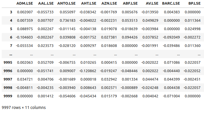
Fig 5: Some of the returns of the stocks from our basket of FTSE100 stocks

Let us now plot the market returns from each stock we have. We can clearly see that certain stocks like Ashtead Group (AHT.LSE) have forceful, strong tails that deviate from the average performance of the portfolio of the 11 stocks we have. In essence, Markowitz's algorithm will help us empirically select less of those stocks that have high variance and select more of the stocks that have less variance. Markowitz's approach is analytical and removes any guess work from the process on our part.

#Let's visualize our market returns
returns.plot()

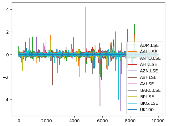
Fig 6: The market returns from our basket of FTSE 100 stocks

Let us observe if there are any meaningful correlation levels in our data. Unfortunately, there were no significant correlation levels that we found interesting.

#Let's analyze the correlation coefficients
fig, ax = plt.subplots(figsize=(8,8)) 
sns.heatmap(returns.corr(),annot=True,linewidths=.5, ax=ax)

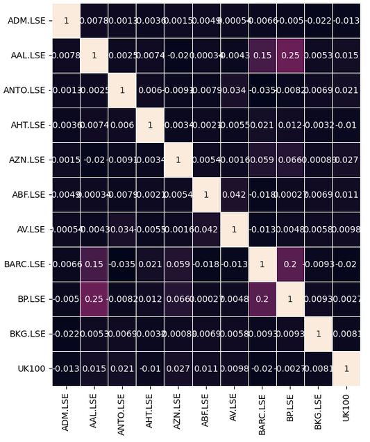
Fig 7: Our correlation heat-map from the FTSE 100

Some relationships will not be easy to find, and require some preprocessing steps to be uncovered. Instead of simply looking for correlation directly between the basket of stocks we have, we can also search for correlation between the current values of each stock, and the future value of the UK100 symbol. This is a classical technique known as lead-lag correlation.

We will start by pushing our basket of stocks backs 20 places, and pushing the UK100 symbol forward 20 places.

# Let's also analyze for lead-lag correlation
look_ahead  = 20
lead_lag    = pd.DataFrame(columns=stocks,index=np.arange(0,returns.shape[0] - look_ahead))
for stock in stocks:
    if stock == 'UK100':
        lead_lag[[stock]] = returns[[stock]].shift(-20)
    else:
        lead_lag[[stock]] = returns[[stock]].shift(20)

# Returns
lead_lag.dropna(inplace=True)

Let us see if there were any changes to the correlation matrix. Unfortunately, we didn't gain any improvements from this procedure.

#Let's see if there are any stocks that are correlated with the future UK100 returns
fig, ax = plt.subplots(figsize=(8,8)) 
sns.heatmap(lead_lag.corr(),annot=True,linewidths=.5, ax=ax)

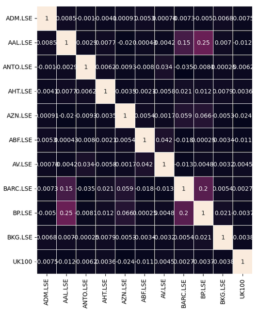
Fig 8: Our lead-lag correlation heat-map

Let us now attempt to minimize the variance of our entire portfolio. We will model our portfolio in such a way that we are allowed to buy and sell different stocks to minimize the risk of our portfolio. To achieve our goal, we will make use of SciPy's optimization library. We will have 11 different weights to be optimized, each weight represents the allocation of capital that must be made to each respective stock. The coefficient of each weight will symbolize whether we should buy, positive coefficient, or sell, negative coefficient, each particular stock. To be more specific, we want to be sure that all our coefficients lie between -1 and 1 inclusive, or in interval notation [-1,1].

On top of this, we would like to use all the capital we have, and no more than that. Therefore, we must set constraints to our optimization procedure. Specifically, we must enforce that the sum of all weights in the portfolio equals 1. This will mean that we have allocated all the capital we have. Recall, that some of our coefficients will be negative, this may make it challenging for the sum of all our coefficients to equal 1. Therefore, we must modify this constraint to only consider the absolute values of each weight. In other words, if we store our 11 weights in a vector, we want to ensure that the L1-norm equals 1.

To get started, we will first initialize our weights with random values and calculate the covariance of our returns' matrix.

#Let's attempt to minimize the variance of the portfolio
weights = np.array([0,0,0,0,0,0,-1,1,1,0,0])
covariance = returns.cov()

Let us now keep track of the initial variance levels.

#Store the initial portfolio variance
initial_portfolio_variance = np.dot(weights.T,np.dot(covariance,weights))
initial_portfolio_variance

0.011959689589562724

When performing optimization, we are looking for the optimal inputs to a function that result in the lowest output from the function. This function is known as the cost function. Our cost function will be the variance of the portfolio under the current weights. Fortunately, this is easy to calculate using linear algebra commands.

#Cost function
def cost_function(x):
    return(np.dot(x.T,np.dot(covariance,x)))

We shall now define our constraints that specify our portfolio weights should equal 1.

#Constraints
def l1_norm(x):
    return(np.sum(np.abs(x))) - 1

constraints = {'type': 'eq', 'fun':l1_norm}

SciPy expects us to provide it with an initial guess when performing optimization.

#Initial guess
initial_guess = weights

Recall that we want our weights to all lie between -1 and 1, we pass these instructions to SciPy using a tuple of bounds.

#Add bounds
bounds =   [(-1,1)] * 11

We will now minimize the variance of our portfolio using the Sequential Least Squares Programming (SLSQP) Algorithm. The SLSQP algorithm was originally developed by accomplished German engineer Dieter Kraft in the 1980s. The original routine was implemented in FORTRAN. Kraft's original scientific paper outlining the algorithm can be found on this link, here. SLSQP is a quasi-newton algorithm, which means that it estimates the second derivative (Hessian matrix) of the objective function to find the optima of the objective function.

#Minimize the portfolio variance
result = minimize(cost_function,initial_guess,method="SLSQP",constraints=constraints,bounds=bounds)

We successfully performed this optimization procedure, let's look at our results.

result

message: Optimization terminated successfully
success: True
status: 0
     fun: 0.0004706570068070814
       x: [ 5.845e-02 -1.057e-01 8.800e-03 2.894e-02 -1.461e-01
            3.433e-02 -2.625e-01 6.867e-02 1.653e-01 3.450e-02
            8.675e-02]
     nit: 12
     jac: [ 3.820e-04 -9.886e-04 3.242e-05 4.724e-04 -1.544e-03
            4.151e-04 -1.351e-03 5.850e-04 8.880e-04 4.457e-04
            4.392e-05]
    nfev: 154
    njev: 12

Let us store the optimal weights our SciPy solver found for us.

#Store the optimal weights
optimal_weights = result.x

Let us validate that the L1-norm constraint was not violated. Note, due to the limited memory floating precision of computers, our weights will not precisely add up to 1.

#Validating the weights add up to one
np.sum(np.abs(optimal_weights))

0.9999999998893961

Store the new portfolio variance.

#Store the new portfolio variance
otpimal_variance = cost_function(optimal_weights)

Create a data-frame to allow us to compare our performance.

#Portfolio variance
portfolio_var = pd.DataFrame(columns=['Old Var','New Var'],index=[0])

Save our variance levels in a data-frame.

portfolio_var.iloc[0,0] = initial_portfolio_variance * (10.0 ** 7)
portfolio_var.iloc[0,1] = otpimal_variance * (10.0 ** 7)

Plot our portfolio variance. As we can see, our variance levels have significantly dropped.

portfolio_var.plot.bar()

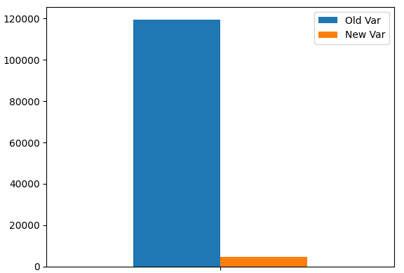
Fig 9:Our new portfolio variance

Let us now obtain the number of positions we should open in each market according to our optimal weights. Our data is suggesting that whenever we open 1 long position in the UK100 symbol, we should open no positions in Admiral Group (ADM.LSE) and we should open 2 equivalent short positions in Anglo-American (AAL.LSE).

int_weights = (optimal_weights / optimal_weights[-1]) // 1
int_weights

array([ 0., -2., 0., 0., -2., 0., -4., 0., 1., 0., 1.])

Updating Our Expert Advisor

Now we can turn our attention to updating our trading algorithm, to take advantage of our new understanding of the FTSE 100 market. Let us first load the optimal weights we calculated using SciPy.

int    optimization_weights[11] = {0,-2,0,0,-2,0,-4,0,1,0,1};

We also need a setting to trigger our optimization procedure, we will set a loss limit. Whenever our open trade's loss is greater than our loss-limit, we will open trades in other FTSE100 markets to try to minimize our risk levels.

input double  loss_limit = 20;        // After how much loss should we optimize our portfolio?

Let us now define the function that will be responsible for calling the procedure for minimizing our portfolio risk levels. Recall, we will only perform this routine if the account has breached its loss limit or is at risk of exceeding its equity threshold.

      //--- Should we optimize our portfolio variance using the optimal weights we have calculated
      if((loss_limit > 0))
        {
         //--- Update the position profit
         position_profit = AccountInfoDouble(ACCOUNT_EQUITY) - AccountInfoDouble(ACCOUNT_BALANCE);
         //--- Check if we have passed our profit target or if we are expecting a reversal
         if(((loss_limit * -1) < position_profit))
           {
            minimize_variance();
           }
        }

This function will actually perform the portfolio optimization, the function will iterate through our list of stocks and then check the number and type of position it should open.

//+------------------------------------------------------------------+
//| This function will minimize the variance of our portfolio        |
//+------------------------------------------------------------------+
void minimize_variance(void)
  {
   risk_minimized = true;

   if(!risk_minimized)
     {
      for(int i = 0; i < 11; i++)
        {
         string current_symbol = list_of_companies[i];

         //--- Add that stock to the portfolio to minimize our variance, buy
         if(optimization_weights[i] > 0)
           {
            for(int i = 0; i < optimization_weights[i]; i++)
              {
               Trade.Buy(0.3,current_symbol,ask,0,0,"FTSE Optimization");
              }
           }
         //--- Add that stock to the portfolio to minimize our variance, sell
         else
            if(optimization_weights[i] < 0)
              {
               for(int i = 0; i < optimization_weights[i]; i--)
                 {
                  Trade.Sell(0.3,current_symbol,bid,0,0,"FTSE Optimization");
                 }
              }
        }
     }
  }

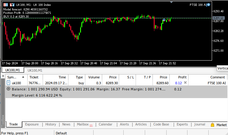
Fig 10: Forward testing our algorithm

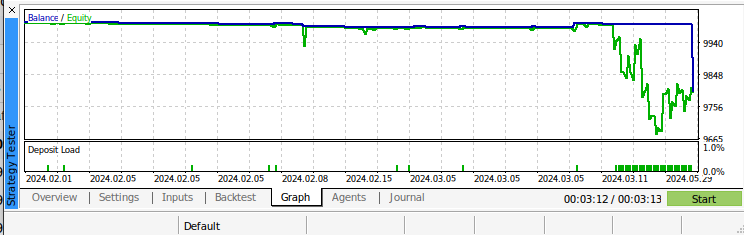
Fig 11: Back testing our algorithm

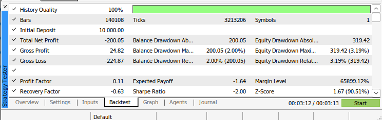
Fig 12:The results from back testing our algorithm

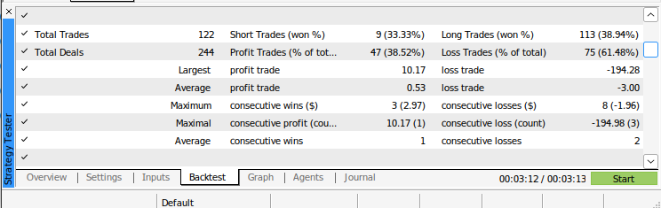
Fig 13: Additional results from back testing our algorithm

Conclusion

In this article, we have demonstrated how you can build an ensemble of technical analysis and AI seamlessly using Python and MQL5, our application is capable of dynamically adjusting itself to all time-frames available in the MetaTrader 5 terminal. We outlined the founding major principles of modern portfolio optimization using contemporary optimization algorithms. We demonstrated how to minimize human bias in the process of portfolio selection. Furthermore, we have showcased how to use market data to make optimal decisions. There is still room for improvement in our algorithm, for example in future articles we will demonstrate how to optimize 2 criteria simultaneously, such as optimizing risk levels while considering the risk free rate of return.

However, most of the principles we have outlined today will remain the same even when we are performing more nuanced optimization procedures, we will only need to adjust our cost functions, constraints and identify the appropriate optimization algorithm for our needs.

Attached files |

Download ZIP

UK100.mq5 (3.16 KB)

Minimizing_Portfolio_Variance.ipynb (369.35 KB)

FTSE_100_AI.mq5 (12.63 KB)

Warning: All rights to these materials are reserved by MetaQuotes Ltd. Copying or reprinting of these materials in whole or in part is prohibited.