Brain Storm Optimization algorithm (Part I): Clustering

Contents

1. Introduction
2. Algorithm description
3. K-Means

1. Introduction

Brain Storm Optimization (BSO) is one of the exciting and innovative population optimization algorithms that is inspired by the natural phenomenon of brainstorming. This optimization method is an effective approach to solving complex problems using the principles of collective intelligence and collective behavior. BSO simulates the process of generating new ideas and solutions, similar to what happens in group discussions, which makes it a unique and promising tool for finding optimal solutions in various areas. In this article, we will look at the basic principles of BSO, its advantages and areas of application.

Population-based methods are an important tool for solving complex optimization problems. However, in the context of multimodal problems where multiple optimal solutions need to be found, existing approaches face limitations. This article presents a new optimization method called the brainstorming optimization method.

Existing approaches, such as niching and clustering methods, typically divide the population into subpopulations to search for multiple solutions. However, these methods suffer from the need to pre-determine the number of subpopulations, which can be challenging, especially when the number of optimal solutions is not known in advance. BSO compensates for this deficiency by transforming the target space into a space where individuals are clustered and updated based on their coordinates. Unlike existing methods that strive for one global optimum, the proposed BSO method directs the search process towards several "meaningful" solutions.

Let's take a closer look at the BSO method and its applicability to multimodal optimization problems. The brainstorming optimization (BSO) algorithm was developed by Shi et al. in 2015. It is inspired by the natural process of brainstorming, when people come together to generate and share ideas to solve a problem.

There are several variants of the algorithm, such as Hypo Variance Brain Storm Optimization, where the estimate of the object function is based on the hypo- or subvariance rather than the Gaussian variance. There are other variants, such as Global-best Brain Storm Optimization, where global best includes a re-initialization scheme triggered by the current state of the population, combined with variable-based updates and fitness-based grouping.

Each individual in the BSO algorithm represents not only a solution to the problem to be optimized, but also a data point that reveals the problem landscape. Collective intelligence and data analysis techniques can be combined to yield benefits beyond what either method could achieve alone.

2. Algorithm

The BSO algorithm works by modeling this process, where a population of candidate solutions (called "individuals" or "ideas") is iteratively updated to converge on an optimal solution. The algorithm consists of the following main stages:

1. Initialization:

- The algorithm starts by generating an initial population of individuals, where each individual represents a potential solution to the optimization problem.
- Each individual is represented by a set of solution variables that define the characteristics of the solution.

2. Brainstorming:

- At this stage, the algorithm simulates brainstorming, where individuals generate new ideas (i.e. new candidate solutions) by combining and modifying their own ideas and the ideas of other individuals.
- Brainstorming is guided by a set of rules that determine how new ideas are generated. These rules are inspired by the human brainstorming and include:

• Random generation of new ideas
• Combination of ideas from different individuals
• Modification of existing ideas

3. Rating:

- Newly generated ideas (i.e. new candidate solutions) are rated using the objective function of the optimization problem.
- The target function measures the quality or fitness of each candidate solution, and the algorithm seeks to find a solution that minimizes (or maximizes) this function.

4. Selection:

- After the rating step, the algorithm selects the best individuals from the population to retain for the next iteration.
- The selection is based on the fitness values of individuals, with fitter individuals having a higher probability of being selected.

5. Completion:

- The algorithm continues to iterate through the brainstorming, rating and selection stages until a termination criterion is met, such as the maximum number of iterations or the achievement of a target solution quality.

Let's list some characteristic BSO methods and algorithm features that distinguish it from other population optimization methods:

1. Clustering. Individuals are grouped into clusters based on their similarity of location in the search space. This is implemented using the K-means clustering algorithm.
2. Convergence. At this stage, individuals within each cluster are grouped around the cluster centroid. This simulates the brainstorming phase, when participants come together to discuss ideas.
3. Divergence. At this stage, new individuals are generated. New individuals can be generated based on one or two individuals in a cluster. This process mimics the brainstorming phase, when participants begin to think outside the box and come up with new ideas.
4. Selection. After new individuals are generated, they are placed into the main parent group, after which the group is sorted. Accordingly, the next iteration will involve handling updated and improved ideas.
5. Mutation. After combining ideas and creating new ones, all newly created ideas are mutated to add additional diversity to the population and prevent premature convergence.

Let's present the logic of the BSO algorithm as pseudocode:

1. Initialization of parameters and generation of the initial population
2. Calculating the fitness of each individual in a population
3. Until the stopping criteria are met:
    4. Calculating the fitness of each individual in a population
    5. Determining the best individual in a population
    6. Splitting the population into clusters, setting the best solution in the cluster as the cluster center
    7. For each new individual in the population:
        |7.1. If the pReplace probability is met:
        |    |a new shifted center of a randomly selected cluster is generated (the cluster center is shifted)
        |7.2. If pOne probability is fulfilled:
        |    |Select a random cluster
        |    |If pOne_center probability is fulfilled:
        |    |    |7.2.a select the cluster center
        |    |Otherwise:
        |         |7.2.b select a random individual from the cluster
        |7.3 Otherwise:
        |         |Select two clusters
        |         |If the pTwo_center probability is fulfilled:
        |             |7.3.a A new individual is formed by merging two cluster centers
        |         |Otherwise:
        |             |7.3.b Create a new individual by merging positions of the selected two individuals from each selected cluster (clusters should be different)
        |7.4 Mutation: Add a random Gaussian deviation to the position of the new individual
        |7.5 If the new individual falls outside the search space, reflect it back into the search space
    8. Update the current population with new individuals
    9. Return to step 4 until the stop criterion is met
10. Return the best individual in the population as a solution
11. End of BSO operation

Let's look at the operations in step 7 of the pseudocode.

The very first operation 7.1, in fact, does not create a new individual, but shifts the center of the cluster, from which new individuals can subsequently be created in other operations of the algorithm. The displacement occurs randomly for each coordinate with a normal distribution at a distance from the original position specified in the external parameters.

Operation 7.2 selects either the cluster center or an individual in the selected cluster that will be mutated in step 7.4 to create the new individual.

Operation 7.3 is designed to create a new individual by merging either the centers of two randomly selected clusters or two individuals from these selected clusters. Clusters should be distinct, but in the case where there is only one non-empty cluster (clusters may be empty), the merge operation is performed on the two selected individuals in this single non-empty cluster. This operation is intended as an exchange of ideas between idea clusters.

The merge operation is as follows:

where:
Xf - new individual after merging,
v - random number from 0 to 1,
X1 and X2 - two random individuals (or two cluster centers) that are to be combined.

The meaning of the merging equation is that an idea will be created at a random location between two other ideas.

The mutation operation can be described by the following equation:

where:
Xm - new individual after mutation,
Xs - selected individual to be mutated,
n(µ, σ) - Gaussian random number with mean µ and variance σ,
ξ - mutation ratio expressed by a mathematical expression.

The mutation ratio is calculated using the equation:

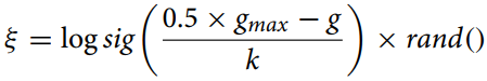
where:
gmax - maximum number of iterations,
g - current iteration number,
k - correction ratio.

This equation (mutation ratio) is used to calculate the shrinking distance between individuals in the optimization algorithm for adaptive change of the mutation parameter. The "logsig()" function provides a smooth non-linear decrease in value and multiplication by "rand" adds a stochastic element that can be useful to avoid premature convergence and maintain population diversity.

The "k" correction ratio in the Brain Storm Optimization (BSO) algorithm plays an important role in controlling the rate of change of the "ξ" ratio over time. The value of "k" may vary depending on the specific problem and data and is calculated empirically or using hyperparameter tuning methods.

In general, "k" should be chosen to provide a balance between exploration and exploitation in the algorithm. If "k" is too big, "ξ" changes very slowly, which may lead to premature convergence of the algorithm. If "k" is too small, "ξ" changes very quickly, which can lead to over-exploration of the search space and slow convergence.

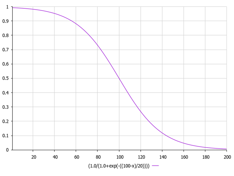
The logarithmic sigmoid function, also known as the logistic function, is commonly denoted as σ(x) or sig(x). It is calculated using the following equation:

where:
exp(-x) - denote the exponent raised to the power of -x.
1 / (1 + exp(-x)) provides an output value in the range from 0 to 1.

The figure below shows the graph of the sigmoid function. Uneven function reduction allows for exploration in early iterations and refinement in later iterations.

Below is an example code for calculating the mutation ratio along with the sigmoid function calculated using the exponential.

In this code, the function "sigmoid" calculates the sigmoid value of the input number "x" and the function "xi" calculates the value of "ξ" according to the equation above. Here "gmax" is the maximum number of iterations, "g" is the current iteration number, and "k" is the correction ratio. The MathRand function generates a random number between 0 and 32 767, so we divide it by 32 767.0 to get a random number between 0 and 1. Then we calculate the sigmoid value of this random number. This value is returned by the "xi" function.

double sigmoid(double x) 
{
    return 1.0 / (1.0 + MathExp(-x));
}

double xi(int gmax, int g, double k) 
{
    double randNum = MathRand() / 32767.0; // Generate a random number from 0 to 1
    return sigmoid (0.5 * (gmax - g) / k) * randNum;
}

3. K-means clustering method

The BSO algorithm uses K-means cluster analysis to separate ideas into distinct groups. The current set of "n" solutions for input into the iteration is divided into "m" categories in order to simulate the behavior of group discussion participants and improve the search efficiency.

We will describe a separate cluster using the S_Cluster structure, which implements the K-means algorithm and is a popular clustering method.

Let's have a look at the structure:

• centroid[] - array representing the cluster centroid.
• f - centroid fitness value.
• count - number of points in the cluster.
• ideasList[] - list of ideas.

The Init function initializes the structure by resizing the "centroid" and "ideasList" arrays and setting the initial value of "f".

//——————————————————————————————————————————————————————————————————————————————
struct S_Cluster
{
    double centroid [];  //cluster centroid
    double f;            //centroid fitness
    int    count;        //number of points in the cluster
    int    ideasList []; //list of ideas

    void Init (int coords)
    {
      ArrayResize (centroid, coords);
      f = -DBL_MAX;
      ArrayResize (ideasList, 0, 100);
    }
};
//——————————————————————————————————————————————————————————————————————————————

The C_BSO_KMeans class is an implementation of the K-means algorithm for clustering agents in the BSO optimization algorithm. Here is what each method does:

1. KMeansInit - method initializes cluster centroids by selecting random agents from the data. For each cluster, a random agent is selected and its coordinates are copied to the cluster centroid.
2. VectorDistance - the method calculates the Euclidean distance between two vectors. It takes two vectors as arguments and returns their Euclidean distance.
3. KMeans - the method implements the basic logic of the k-means algorithm for data clustering. It takes the data and cluster arrays as arguments.

The K-means method performs the following steps during operation:

• Assigning data points to the nearest centroid.
• Update centroids based on the mean of the points assigned to each cluster.
• Repeat these two steps until the centroids stop changing or the maximum number of iterations is reached.

Centroid in the K-means clustering method is a central pointer of the cluster. In the context of the K-means method, the centroid is the arithmetic mean of all data points belonging to a given cluster.
In each iteration of the K-means algorithm, the centroids are recalculated, after which the data points are again grouped into clusters according to which of the new centroids was closer according to the chosen metric.
Thus, centroids play a key role in the K-means method, determining the shape and position of clusters.

This class represents a key part of the BSO optimization algorithm, providing clustering of agents to improve the search process. The K-means algorithm iteratively assigns points to clusters and recalculates centroids until no more changes occur or the maximum number of iterations is reached.

//——————————————————————————————————————————————————————————————————————————————
class C_BSO_KMeans
{
  public: //--------------------------------------------------------------------

  void KMeansInit (S_BSO_Agent &data [], int dataSizeClust, S_Clusters &clust [])
  {
    for (int i = 0; i < ArraySize (clust); i++)
    {
      int ind = MathRand () % dataSizeClust;
      ArrayCopy (clust [i].centroid, data [ind].c, 0, 0, WHOLE_ARRAY);
    }
  }

  double VectorDistance (double &v1 [], double &v2 [])
  {
    double distance = 0.0;
    for (int i = 0; i < ArraySize (v1); i++)
    {
      distance += (v1 [i] - v2 [i]) * (v1 [i] - v2 [i]);
    }
    return MathSqrt (distance);
  }

  void KMeans (S_BSO_Agent &data [], int dataSizeClust, S_Clusters &clust [])
  {
    bool changed   = true;
    int  nClusters = ArraySize (clust);
    int  cnt       = 0;

    while (changed && cnt < 100)
    {
      cnt++;
      changed = false;

      //Assigning data points to the nearest centroid
      for (int d = 0; d < dataSizeClust; d++)
      {
        int    closest_centroid = -1;
        double closest_distance = DBL_MAX;

        if (data [d].f != -DBL_MAX)
        {
          for (int cl = 0; cl < nClusters; cl++)
          {
            double distance = VectorDistance (data [d].c, clust [cl].centroid);

            if (distance < closest_distance)
            {
              closest_distance = distance;
              closest_centroid = cl;
            }
          }

          if (data [d].label != closest_centroid)
          {
            data [d].label = closest_centroid;
            changed = true;
          }
        }
        else
        {
          data [d].label = -1;
        }
      }


      //Updating centroids
      double sum_c [];
      ArrayResize (sum_c, ArraySize (data [0].c));

      for (int cl = 0; cl < nClusters; cl++)
      {
        ArrayInitialize (sum_c, 0.0);

        clust [cl].count = 0;
        ArrayResize (clust [cl].ideasList, 0);

        for (int d = 0; d < dataSizeClust; d++)
        {
          if (data [d].label == cl)
          {
            for (int k = 0; k < ArraySize (data [d].c); k++)
            {
              sum_c [k] += data [d].c [k];
            }

            clust [cl].count++;
            ArrayResize (clust [cl].ideasList, clust [cl].count);
            clust [cl].ideasList [clust [cl].count - 1] = d;
          }
        }

        if (clust [cl].count > 0)
        {
          for (int k = 0; k < ArraySize (sum_c); k++)
          {
            clust [cl].centroid [k] = sum_c [k] / clust [cl].count;
          }
        }
      }
    }
  }
};
//——————————————————————————————————————————————————————————————————————————————

In the Brain Storm Optimization (BSO) algorithm, the fitness of an individual is defined as the quality of the solution it represents. In an optimization problem, the fitness can be equal to the value of the function being optimized.

The specific clustering method may vary. One common approach is to use the k-means method, where cluster centroids are initialized randomly and then iteratively updated to minimize the sum of the squared distances from each point to its cluster centroid.

Although fitness plays a key role in clustering, it is not the only factor that influences cluster formation. Other aspects, such as the distance between individuals in the decision space, may also play an important role. This helps the algorithm maintain diversity in the population and prevent premature convergence to inappropriate solutions.

The number of iterations required for the K-means algorithm to converge depends heavily on various factors, such as the initial state of the centroids, the distribution of the data, and the number of clusters. However, in general, K-means typically converges in a few tens to a few hundred iterations.

It is also worth considering that K-means minimizes the sum of squared distances from points to their closest centroids, which may not always be optimal depending on the specific task and the shape of the clusters in the data. In some cases, other clustering algorithms may be more appropriate.

K-means++ is an improved version of the K-means algorithm proposed in 2007 by David Arthur and Sergei Vassilvitskii. The main difference between K-means++ and standard K-means is the way the centroids are initialized. Instead of randomly choosing initial centroids, K-means++ chooses them in such a way as to maximize the distance between them. This helps to improve the quality of clustering and speeds up the convergence of the algorithm.

Here are the main initialization steps in K-means++:

1. Randomly select the first centroid from the data points.
2. For each data point, calculate its distance to the nearest, previously selected centroid.
3. Select the next centroid from the data points such that the probability of selecting a point as a centroid is directly proportional to its distance from the closest, previously selected centroid (that is, the point that has the maximum distance to the nearest centroid is most likely to be chosen as the next centroid).
4. Repeat steps 2 and 3 until k centroids have been selected.

After initializing the centroids, K-means++ continues to operate in the same way as the standard one. This initialization method helps to improve the quality of clustering and speeds up the convergence of the algorithm. However, this method is computationally expensive.

If you have 1000 coordinates for each point, this will create additional computational overhead for the K-means++ algorithm, since it has to calculate distances in a high-dimensional space. However, K-means++ may still be effective (experiments are needed to confirm this assumption), as it usually results in faster convergence and better cluster quality.

When working with high-dimensional data (such as 1000 coordinates), additional problems associated with the "curse of dimensionality" may arise. This can make the distances between points less meaningful and make clustering difficult. In such cases, it may be useful to use dimensionality reduction methods such as PCA (Principal Component Analysis) before applying K-means or K-means++. This can help reduce the dimensionality of the data and make clustering more efficient.

Data dimensionality reduction is an important step in data processing, especially when working with a large number of coordinates or features. This helps to simplify data, reduce computational costs and improve the performance of clustering algorithms. Here are some dimensionality reduction methods that are often used in clustering:

1. Principal Component Analysis (PCA). This method transforms a data set with a large number of variables into a data set with fewer variables while retaining the maximum amount of information.
2. Multidimensional scaling (MDS). The method attempts to find a low-dimensional structure that preserves the distances between points as in the original high-dimensional space.
3. t-distributed Stochastic Neighbor Embedding (t-SNE). It is a non-linear dimensionality reduction method that is particularly good for visualizing high-dimensional data.
4. Autoencoders. These are neural networks that are used to reduce the dimensionality of data. They work by learning to encode input data into a compact representation, and then decode that representation back into the original data.
5. Independent Component Analysis (ICA). This is a statistical method that transforms a data set into independent components that may be more informative than the original data. The components may better reflect the structure or important aspects of the data, for example, they may make some hidden factors visible or allow better separation of classes in a classification problem.
6. Linear Discriminant Analysis (LDA). The method is used to find linear combinations of features that separate two or more classes well.

So, although K-means++ may be more computationally expensive during the initialization step, especially for high-dimensional data, it may still be worthwhile in some cases. But it is always worth experimenting and comparing different approaches to determine what works best for your particular problem and dataset.

In case you would like to experiment further with the K-means++ method, here is the initialization method for this algorithm (the rest of the code is no different from the conventional K-means code).

The code below is an implementation of the K-means++ algorithm initialization. The function takes an array of data points represented by the S_BSO_Agent structure, a data size (dataSizeClust) and an array of clusters represented by the S_Cluster structure. The method initializes the first centroid randomly from the data points. Then, for each subsequent centroid, the algorithm calculates the distance from each data point to the closest centroid and chooses the next centroid with a probability proportional to the distance. This is done by generating a random number "r" between 0 and the sum of all distances, and then looping through all the data points, decreasing "r" by the distance of each point until "r" is less than or equal to the distance of the current point. In this case, the current point is chosen as the next centroid. This process is repeated until all centroids are initialized.

Overall, K-Means++ initialization is implemented, which is an improved version of the initialization in the standard K-Means algorithm. The centroids are chosen to minimize the potential sum of squared distances between the centroids and the data points, leading to more efficient and stable clustering.

void KMeansPlusPlusInit (S_BSO_Agent &data [], int dataSizeClust, S_Cluster &clust [])
{
  // Choose the first centroid randomly
  int ind = MathRand () % dataSizeClust;
  ArrayCopy (clust [0].centroid, data [ind].c, 0, 0, WHOLE_ARRAY);

  for (int i = 1; i < ArraySize (clust); i++)
  {
    double sum = 0;
      
    // Compute the distance from each data point to the nearest centroid
    for (int j = 0; j < dataSizeClust; j++)
    {
      double minDist = DBL_MAX;
       
      for (int k = 0; k < i; k++)
      {
        double dist = VectorDistance (data [j].c, clust [k].centroid);
          
        if (dist < minDist)
        {
            minDist = dist;
        }
      }
        
      data [j].minDist = minDist;
      sum += minDist;
    }

    // Choose the next centroid with a probability proportional to the distance
    double r = MathRand () * sum;
      
    for (int j = 0; j < dataSizeClust; j++)
    {
      if (r <= data [j].minDist)
      {
        ArrayCopy (clust [i].centroid, data [j].c, 0, 0, WHOLE_ARRAY);
        break;
      }
      r -= data [j].minDist;
    }
  }
}

To be continued...

In this article, we examined the logical structure of the BSO algorithm, as well as clustering methods and ways to reduce the dimensionality of the optimization problem. In the next article, we will complete our study of the BSO algorithm and summarize its performance.