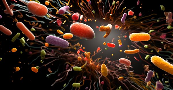
Population optimization algorithms: Bacterial Foraging Optimization - Genetic Algorithm (BFO-GA)

Contents

1. Introduction
2. Algorithm
3. Test results

1. Introduction

The BFO-GA hybrid optimization algorithm combines two different optimization algorithms: the foraging optimization (BFO) algorithm and the genetic algorithm (GA). This hybrid algorithm was created to improve optimization efficiency and overcome some of the shortcomings of each of the individual algorithms.

BFO (Bacterial Foraging Optimization) is an optimization algorithm inspired by the foraging behavior of bacteria. It was proposed in 2002 by Rahul K. Kujur. BFO models bacterial movement using three main mechanisms: transitions, diffusion, and position update. Each bacterium in the algorithm represents a solution to the optimization problem, and food corresponds to the optimal solution. Bacteria move through search space to find the best food.

Genetic algorithm (GA) is an optimization algorithm inspired by the principles of natural selection and genetics. It was developed by John Holland in the 1970s. GA works with a population of individuals representing solutions to an optimization problem. Individuals undergo the operations of crossing (combining genetic information) and mutation (random changes in genetic information) to create new generations. After several generations, GA strives to find the optimal solution.

The hybrid BFO-GA algorithm combines the advantages of both algorithms. BFO has good local search and fast convergence capabilities, but may struggle with global search. On the other hand, GA has good global search ability, but can be slow in convergence and prone to getting stuck in local optima. The hybrid BFO-GA algorithm attempts to overcome these limitations by using BFO for global search and GA for refining local optima.

The BFO-GA (Bacterial Foraging Optimization - Genetic Algorithm) hybrid algorithm was proposed in 2007 by D. N. Kim, A. Abraham and Chow. This algorithm combines optimization principles based on the behavior of swarming bacteria with genetic operators of selection, crossover and mutation.

BFO-GA uses the bacterial algorithm as a basis, but extends it with genetic selection, crossover, and mutation operators. This algorithm uses bacterial swarming to find the optimal solution.

BFO-GA uses an algorithm based on the roulette method as the selection operator. This method selects parent bacteria with probabilities proportional to their fitness. Thus, fitter bacteria are more likely to be selected for interbreeding.

Crossing in the BFO-GA algorithm is implemented using the arithmetic crossover operator. It combines the genetic information of the two parent bacteria, creating new offspring with new gene combinations.

Mutation in BFO-GA is performed using the non-uniform Mihaljevic mutator. This mutator changes the genetic information within bacteria making random changes. Unevenness of mutation means that the probability of mutation can vary depending on various factors.

These modifying operators are performed after completion of the chemotaxis and reproduction procedures of the bacterial algorithm before the elimination and dispersal procedures of this algorithm. In other words, after the bacteria have moved towards the optimal solution and produced offspring, genetic operators are applied to diversify and improve solutions.

2. Algorithm

The BFO-GA algorithm uses modeling of the behavior of swarming bacteria to find the optimal solution to an optimization problem. It simulates the movement of bacteria in parameter space, where each bacterium represents a potential solution to a problem. Bacteria move through parameter space by performing two main types of movements: movement in the direction of a nutritional gradient and movement in a random direction.

The BFO-GA algorithm uses the following steps:

1. Initialization: Creation of an initial population of bacteria, each of which represents a potential solution to a problem. Each bacterium has its own parameters that can be changed during the optimization process.
2. Nutritional Gradient Estimation: Calculating the fitness function value for each bacterium in a population and then comparing the last two values, and this difference in value determines the quality of the solution presented by each bacterium.
3. Movement in the direction of the gradient: Each bacterium moves in the direction of the food gradient, which allows it to move towards more optimal solutions with a constant vector of change in position.
4. Movement in a random direction: Some bacteria also perform random movement to avoid getting stuck in local optima. This movement is based on a random change in the parameters of the bacterium in the event of a previous unsuccessful movement.
5. Genetic operators: Application of genetic operators - selection, crossing and mutation, to a population of bacteria. This allows us to create new combinations of parameters and improve the quality of solutions.
6. Repeating steps 2-5: Repeating the steps of moving in the gradient direction, moving in the random direction and applying genetic operators until a stop criterion is reached, such as reaching the maximum number of iterations or reaching a certain fitness function value.

In theory, the hybrid BFO-GA algorithm should have a number of advantages over BFO that are worth mentioning:

1. Exploration and exploitation: BFO-GA has the ability to explore the parameter space due to the random movement of bacteria, and exploitation due to movement in the direction of the food gradient. This allows the algorithm to find optimal solutions by avoiding local optima and converging to a global one.
2. Adaptability: BFO-GA has the ability to adapt to changing optimization conditions. During the algorithm operation, the parameters of the bacteria can change, which allows them to adapt to new conditions and find more optimal solutions.
3. No need for parameter tuning: Like any optimization algorithm, BFO-GA has a set of parameters that can be tuned to achieve better results. This includes parameters related to the size of the bacterial population, steps of movement in the direction of the gradient and random movement, probabilities of genetic operators and others. Changing the parameters does not have a significant effect on the result.
   

Figure 1. Inheritance of parental "genes" by daughter bacteria

Let's move from theoretical foundations to practical implementation.

First, I abandoned selection using the roulette method (the method was used in the artificial bee colony algorithm ). Experiments yielded better results in BFO-GA with the use of simple random sampling from a parental population.

Second, I decided to replace the non-uniform Mihaljevic mutator with a power law mutation (in some sources, it is referred to as a type of power law mutator). In fact, this is a generation of a random number with a power law distribution, mentioned in the article about Smart Cephalopod.

Third, the arithmetic crossover operator is replaced by simple random inheritance of genes from different parents selected at random according to a uniform distribution law.

To describe a bacterium, we will write the S_Bacteria structure containing the following fields:

• c: array of bacteria coordinates represents the current coordinates of the bacteria in parameter space. The size of the "c" array depends on the number of variables in the optimization problem.
• cLast: array of previous coordinates of the bacterium used to store the previous position of the bacterium in the space of parameters the new position is calculated from.
  
• v: array of bacteria vectors represents the current direction of movement of the bacteria in parameter space. The size of the "v" array depends on the number of variables in the optimization problem.
• f: the current value of the bacterium health (fitness) determines the quality of the current position of the bacterium in the parameter space. The larger the "f" value, the better.
• fLast: previous health value of the bacterium used to track the previous quality of the bacterium's position and applied in determining the nutritional gradient.
  
• lifeCNT: bacteria life counter tracks the number of iterations the bacterium has spent in its current position. The field is used to limit the number of steps bacteria can take in one direction.
  

//——————————————————————————————————————————————————————————————————————————————
struct S_Bacteria
{
  double c     []; //coordinates
  double cLast []; //coordinates
  double v     []; //vector
  double f;        //current health
  double fLast;    //previous health
  double lifeCNT;  //life counter
};
//——————————————————————————————————————————————————————————————————————————————

Declare the C_AO_BFO_GA class, which implements the BFO-GA algorithm. Let's look at each field and class method:

Class fields:

• b: array of bacteria. Each element of the array is an object of "S_Bacteria" type representing a bacterium in the algorithm.
• rangeMax: array of maximum search range values for each variable in the optimization problem.
• rangeMin: array of minimum search range values for each variable.
• rangeStep: array of search steps for each variable.
• cB: array of best coordinates found by the algorithm.
• fB: fitness function value for the best coordinates.

Class methods:

• Init: Initializes the parameters of the BFO-GA algorithm, such as "paramsP" (number of optimized parameters), "populationSizeP" (population size), "lambda" (bacteria movement length), "reproductionP" (reproduction probability), "lifeCounterP" (life counter) - upon completion of the number of lives, bacteria perform a somersault, and "powerMutP" (mutation power).
• Swimming: carries out the movement of bacteria in parameter space.
• Evaluation: population revision and global solution update.
  

Private class methods:

• NewVector: generates a new vector for the specified "paramInd" bacterium parameter.
• PowerDistribution: applies a power distribution to the In input with the specified "outMin", "outMax" and "power" parameters.
• Sorting: sorts bacteria in a population by their fitness function values in descending order.
• SeInDiSp: normalizes the In input in the [InMin, InMax] interval with "Step".
• RNDfromCI: generates a random number in a given [min, max] interval.
• Scale: scales the In input from the [InMIN, InMAX] interval to the [OutMIN, OutMAX] interval.
  

//——————————————————————————————————————————————————————————————————————————————
class C_AO_BFO_GA
{
  //----------------------------------------------------------------------------
  public: S_Bacteria b     []; //bacteria
  public: double rangeMax  []; //maximum search range
  public: double rangeMin  []; //manimum search range
  public: double rangeStep []; //step search
  public: double cB        []; //best coordinates
  public: double fB;           //FF of the best coordinates

  public: void Init (const int    paramsP,         //number of opt. parameters
                     const int    populationSizeP, //population size
                     const double lambdaP,         //lambda
                     const double reproductionP,   //probability of reproduction
                     const int    lifeCounterP,    //life counter
                     const double powerMutP);      //mutation power

  public: void Swimming   ();
  public: void Evaluation ();

  //----------------------------------------------------------------------------
  private: double NewVector (int paramInd);
  private: S_Bacteria bT []; //bacteria
  private: double v      [];
  private: int    ind    [];
  private: double val    [];

  private: int    populationSize; //population size
  private: int    parameters;     //number of optimized parameters
  private: double lambda;         //lambda
  private: double reproduction;   //probability of reproduction
  private: int    lifeCounter;    //life counter
  private: double powerMut;       //mutation power
  private: bool   evaluation;

  private: double PowerDistribution (const double In, const double outMin, const double outMax, const double power);
  private: void   Sorting           ();
  private: double SeInDiSp          (double In, double InMin, double InMax, double Step);
  private: double RNDfromCI         (double min, double max);
  private: double Scale             (double In, double InMIN, double InMAX, double OutMIN, double OutMAX,  bool revers);
};
//——————————————————————————————————————————————————————————————————————————————

The Init method is used to initialize the class. The method initializes the parameters of the BFO-GA algorithm.

Method inputs:

• paramsP: number of optimized parameters.
• populationSizeP: population size.
• lambdaP: lambda parameter that determines the distance the bacteria move at each step.
  
• reproductionP: reproduction probability.
• lifeCounterP: life counter.
• powerMutP: mutation power.

Inside the method, the fields of the C_AO_BFO_GA class are initialized with initial values and the array sizes are set.

//——————————————————————————————————————————————————————————————————————————————
void C_AO_BFO_GA::Init (const int    paramsP,         //number of opt. parameters
                        const int    populationSizeP, //population size
                        const double lambdaP,         //lambda
                        const double reproductionP,   //probability of reproduction
                        const int    lifeCounterP,    //life counter
                        const double powerMutP)       //mutation power
{
  fB = -DBL_MAX;
  evaluation = false;

  parameters      = paramsP;
  populationSize  = populationSizeP;
  lambda          = lambdaP;
  reproduction    = reproductionP;
  lifeCounter     = lifeCounterP;
  powerMut        = powerMutP;

  ArrayResize (rangeMax,  parameters);
  ArrayResize (rangeMin,  parameters);
  ArrayResize (rangeStep, parameters);
  ArrayResize (v,         parameters);

  ArrayResize (ind,       populationSize);
  ArrayResize (val,       populationSize);

  ArrayResize (b,  populationSize);
  ArrayResize (bT, populationSize);

  for (int i = 0; i < populationSize; i++)
  {
    ArrayResize (b [i].c,     parameters);
    ArrayResize (b [i].cLast, parameters);
    ArrayResize (b [i].v,     parameters);
    b [i].f     = -DBL_MAX;
    b [i].fLast = -DBL_MAX;

    ArrayResize (bT [i].c,     parameters);
    ArrayResize (bT [i].cLast, parameters);
    ArrayResize (bT [i].v,     parameters);
  }

  ArrayResize (cB, parameters);
}
//——————————————————————————————————————————————————————————————————————————————

Write the Swimming method to carry out the hemitaxis of bacteria, their replication, selection, inheritance of characteristics and mutation:

void Swimming ()
{
}

At the first iteration, the "evaluation" flag is equal to "false". Distribute the bacteria throughout the entire search space randomly with a uniform distribution. At this stage, the current health (fitness) and the previous one are unknown. Let's assign the DBL_MAX value to the corresponding variables. Also, add a random movement vector to the newly created bacteria.

Check the bacteria coordinates for going beyond the boundaries and apply the step of changing the optimized parameters. The movement vector of each bacterium allows them to swim uniformly forward.

if (!evaluation)
{
  fB = -DBL_MAX;

  for (int s = 0; s < populationSize; s++)
  {
    for (int k = 0; k < parameters; k++)
    {
      b [s].c [k] = RNDfromCI (rangeMin [k], rangeMax [k]);
      b [s].c [k] = SeInDiSp (b [s].c [k], rangeMin [k], rangeMax [k], rangeStep [k]);

      v [k] = rangeMax [k] - rangeMin [k];

      b [s].v [k] = NewVector (k);

      b [s].f     = -DBL_MAX;
      b [s].fLast = -DBL_MAX;

      b [s].lifeCNT = 0;
    }
  }

  evaluation = true;
  return;
}

The probability of reproduction (replication) of bacteria is first checked at the second and subsequent iterations. If the probability of reproduction is fulfilled, then the following happens:

• "bacterium original": the best half of the sorted bacterial population continues its movement in the same direction. To do this, we add a movement vector individual for each bacterium to the coordinates of the previous position.
  
•  "bacterium clone": the second half of the population is filled with daughter bacteria obtained from the "genes" (coordinates) of different parent bacteria. Thus, they inherit characteristics and fulfill the combinatorial ability of the algorithm (see Figure 1 above).
  
• Cloned bacteria that have inherited genes from different parents also inherit a component of the parent's motion vector, and the inherited gene undergoes mutation according to a power law distribution.

Thus, cloned bacteria inherit the characteristics of different parents. In this case, genes change with high probability in their vicinity. The probability decreases with the increasing distance from the values of the parent gene. This allows us to combine the successful properties of parents, since only the best members of the population can pass on genes to their heirs. In addition, the inherited components of the movement vector cause the daughter bacteria to move in the next iteration in accordance with the best components of the parental vectors.

Ideally, this should resemble the movement of a school of fish, but this analogy is not always confirmed due to the influence of many random factors on the movement of bacteria. Such factors include the landscape of fitness function, replacement by more fortunate members of the population and the inevitable change in the vector of movement due to the limitation of the number of lives.

The life counter of bacteria in the better half of the colony increases by one, while for cloned ones it is reset.

double r = RNDfromCI (0.0, 1.0);

if (r < reproduction)
{
  int st = populationSize / 2;

  //bacterium original--------------------------------------------------------
  for (int s = 0; s < st; s++)
  {
    for (int k = 0; k < parameters; k++)
    {
      b [s].c [k] = b [s].cLast [k] + b [s].v [k];
      b [s].c [k] = SeInDiSp (b [s].c [k], rangeMin [k], rangeMax [k], rangeStep [k]);
    }
    b [s].lifeCNT++;
  }

  //bacterium clone-----------------------------------------------------------
  for (int s = st; s < populationSize; s++)
  {
    for (int k = 0; k < parameters; k++)
    {
      int i = (int)RNDfromCI (0, st);
      if (i >= st) i = st - 1;

      b [s].c [k] = b [i].cLast [k];

      b [s].c [k] = PowerDistribution (b [s].c [k], rangeMin [k], rangeMax [k], powerMut);
      b [s].c [k] = SeInDiSp (b [s].c [k], rangeMin [k], rangeMax [k], rangeStep [k]);
    }
    b [s].lifeCNT = 0;
  }
}

Next, if the probability of reproduction is not satisfied, in the loop for the entire population:

for (int s = 0; s < populationSize; s++)

A check for reaching the limit of bacterial lives is performed first. Having reached the limit of lives, bacteria do somersaults and begin to move in a new direction changing their movement vector. The life counter is reset.

After checking for the bacteria to reach the life limit, those who have reached it mutate, and at the next iteration they begin to move in a new direction, changing their movement vector. The life counter is reset.

if (b [s].lifeCNT >= lifeCounter)
{
  for (int k = 0; k < parameters; k++)
  {
    b [s].v [k] = NewVector (k);

    b [s].c [k] = PowerDistribution (b [s].cLast [k], rangeMin [k], rangeMax [k], powerMut);
    b [s].c [k] = SeInDiSp (b [s].c [k], rangeMin [k], rangeMax [k], rangeStep [k]);
  }
  b [s].lifeCNT = 0;
}

If the bacterium has not yet reached its life limit, we check for positive chemotaxis, that is, whether the bacterium is moving towards an increasing food gradient. The movement of the bacterium is considered correct if the fitness values in the two previous iterations are equal. Why exactly equal? At the next stage, in the Evaluation method, we check for a positive change in the health of bacteria. If the changes are positive, then the current state is assigned to the previous state. If the health states in the last two iterations are the same, this indicates that the direction of the bacteria movement in search of more food is correct. Thus, the bacterium can only move towards more food. Otherwise, the bacteria begins to tumble in place. However, this is not a problem, since sooner or later the stuck bacterium will either mutate into a new state or inherit the genes of more fortunate parents and their vector of movement.

The life counter of bacteria moving in the right direction gradually increases. This means that sooner or later even successful bacteria will undergo mutations, as mentioned in the previous code block.

if (b [s].f == b [s].fLast)
{
  for (int k = 0; k < parameters; k++)
  {
    b [s].c [k] = b [s].cLast [k] + b [s].v [k];
    b [s].c [k] = SeInDiSp (b [s].c [k], rangeMin [k], rangeMax [k], rangeStep [k]);
  }
  b [s].lifeCNT++;
}

If positive chemotaxis is not observed in a bacterium, then such a bacterium changes the vector of movement making a somersault. The life counter of such bacteria also continues to tick. The idea arose to increase the value of the life counter of such unsuccessful bacteria more intensively, although I have not tested this idea.

for (int k = 0; k < parameters; k++)
{
  b [s].v [k] = NewVector (k);
  b [s].c [k] = b [s].cLast [k] + b [s].v [k];
  b [s].c [k] = SeInDiSp (b [s].c [k], rangeMin [k], rangeMax [k], rangeStep [k]);
}
b [s].lifeCNT++;

To perform a somersault (change the motion vector), use the NewVector method, which is executed for the optimized parameter with the "paramInd" index:

• a random number "r" is generated with a uniform distribution in the [-1.0, 1.0] interval using the "RNDfromCI" function.
• a new value of the vector component is calculated by multiplying the permissible "v" range of values of the optimized parameter by the "lambda" ratio and the "r" random number.

//——————————————————————————————————————————————————————————————————————————————
double C_AO_BFO_GA::NewVector (int paramInd)
{
  double r = RNDfromCI (-1.0, 1.0);
  return lambda * v [paramInd] * r;
}
//——————————————————————————————————————————————————————————————————————————————

The Evaluation method is used to arrange the competition between bacteria and update the global solution.

At the beginning of the method, each bacterium in the population is tested for the positive chemotaxis: if the current value of the fitness function "b[s].f" is greater than the previous value "b[s].fLast", the previous fitness and coordinates (the bacteria will move from) are updated.

The population is then sorted using the Sorting method in descending order of fitness function values using the fLast value of the bacteria.

After this, the global solution is updated.

//——————————————————————————————————————————————————————————————————————————————
void C_AO_BFO_GA::Evaluation ()
{
  for (int s = 0; s < populationSize; s++)
  {
    if (b [s].f > b [s].fLast)
    {
      b [s].fLast = b [s].f;
      ArrayCopy (b [s].cLast, b [s].c, 0, 0, WHOLE_ARRAY);
    }
  }

  Sorting ();

  if (b [0].fLast > fB)
  {
    fB = b [0].fLast;
    ArrayCopy (cB, b [0].cLast, 0, 0, WHOLE_ARRAY);
  }
}
//——————————————————————————————————————————————————————————————————————————————

3. Test results

BFO-GA test stand results:

C_AO_BFO_GA:50;0.01;0.8;50;10.0
=============================
5 Hilly's; Func runs: 10000; result: 0.8914957961234459
25 Hilly's; Func runs: 10000; result: 0.5511088047221568
500 Hilly's; Func runs: 10000; result: 0.31529201642392934
=============================
5 Forest's; Func runs: 10000; result: 0.9698155977381523
25 Forest's; Func runs: 10000; result: 0.39612322805995287
500 Forest's; Func runs: 10000; result: 0.06304955092899359
=============================
5 Megacity's; Func runs: 10000; result: 0.7266666666666667
25 Megacity's; Func runs: 10000; result: 0.275
500 Megacity's; Func runs: 10000; result: 0.035250000000000004
=============================
All score: 4.22380 (46.93%)

A visual analysis of the test stand operation shows that the BFO-GA algorithm quickly detects the area of the global extremum, while paying less attention to the study of local extrema, which could potentially lead to getting stuck if the global extremum turns out to be erroneous. In general, the algorithm converges quite reliably, although somewhat slowly. Some "swarming" is observed, which is a good sign, but there is no complete communication between the bacteria, and they behave as independent population units.

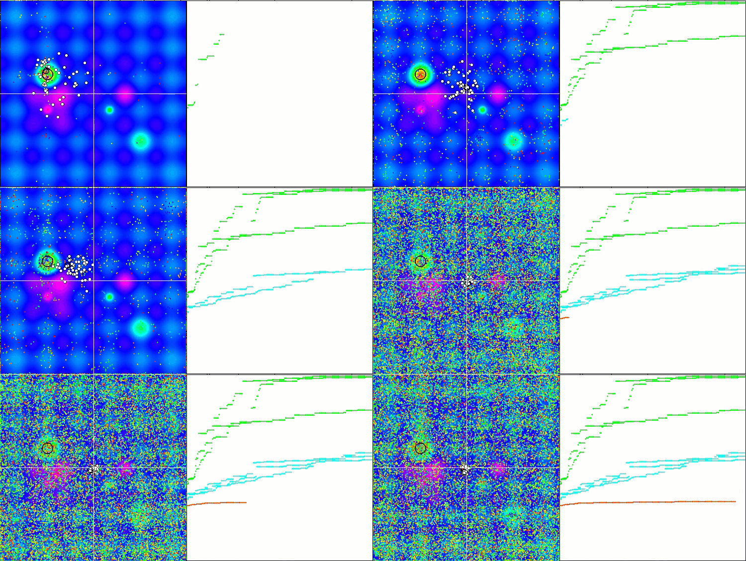
  BFO-GA on the Hilly test function

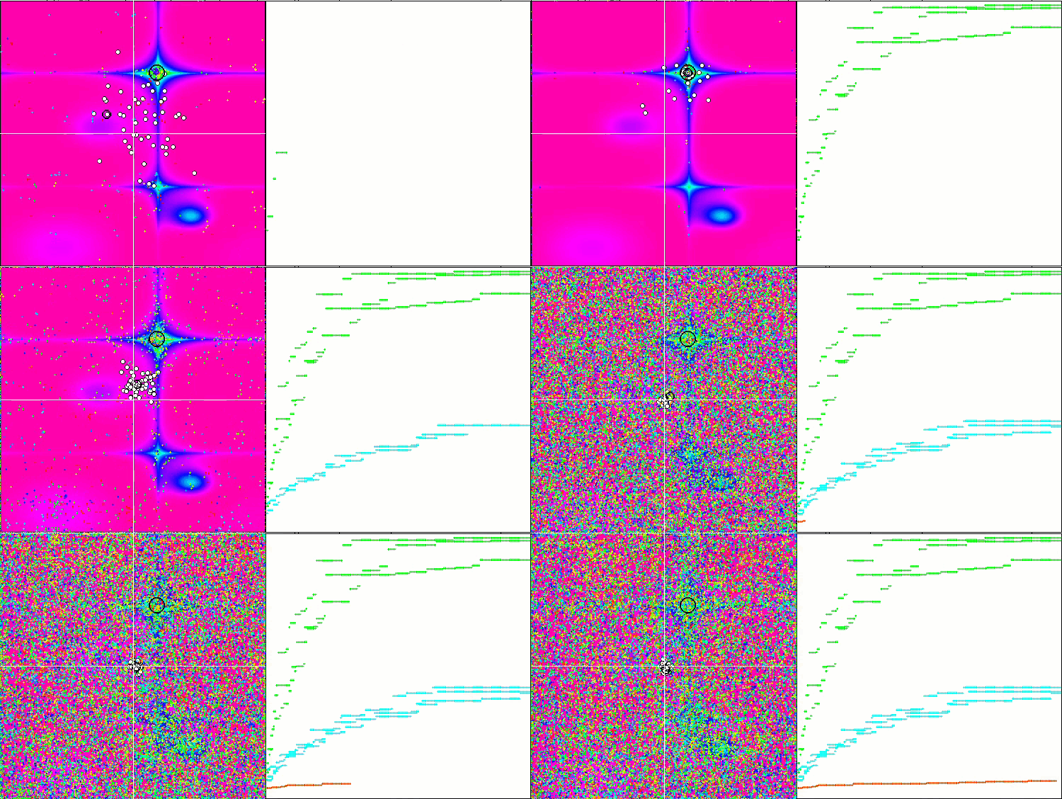
  BFO-GA on the Forest test function

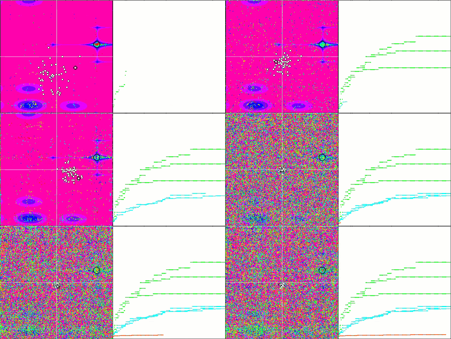
  BFO-GA on the Megacity test function

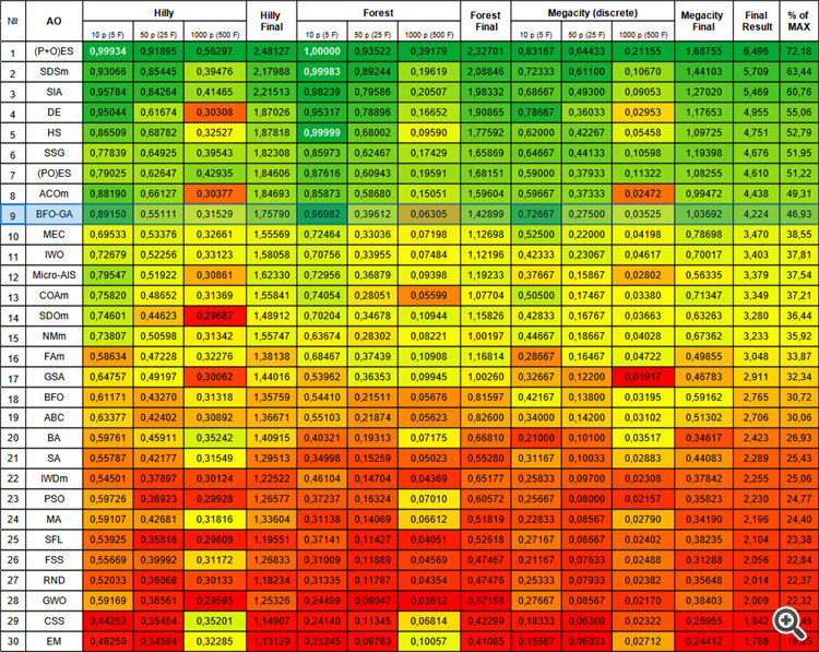
In the overall rating table, the BFO-GA algorithm takes the 9 th place, which is a fairly high result. This indicates that the transformations made when adding genetic algorithm operators to the original BFO algorithm were not in vain and led to appropriate results. This algorithm demonstrated predominantly the best results on test functions with a small number of variables surpassing most other algorithms.

#	AO	Description	Hilly			Hilly final	Forest			Forest final	Megacity (discrete)			Megacity final	Final result	% of MAX
			10 p (5 F)	50 p (25 F)	1000 p (500 F)		10 p (5 F)	50 p (25 F)	1000 p (500 F)		10 p (5 F)	50 p (25 F)	1000 p (500 F)
1	(P+O)ES	(P+O) evolution strategies	0.99934	0.91895	0.56297	2.48127	1.00000	0.93522	0.39179	2.32701	0.83167	0.64433	0.21155	1.68755	6.496	72.18
2	SDSm	stochastic diffusion search M	0.93066	0.85445	0.39476	2.17988	0.99983	0.89244	0.19619	2.08846	0.72333	0.61100	0.10670	1.44103	5.709	63.44
3	SIA	simulated isotropic annealing	0.95784	0.84264	0.41465	2.21513	0.98239	0.79586	0.20507	1.98332	0.68667	0.49300	0.09053	1.27020	5.469	60.76
4	DE	differential evolution	0.95044	0.61674	0.30308	1.87026	0.95317	0.78896	0.16652	1.90865	0.78667	0.36033	0.02953	1.17653	4.955	55.06
5	HS	harmony search	0.86509	0.68782	0.32527	1.87818	0.99999	0.68002	0.09590	1.77592	0.62000	0.42267	0.05458	1.09725	4.751	52.79
6	SSG	saplings sowing and growing	0.77839	0.64925	0.39543	1.82308	0.85973	0.62467	0.17429	1.65869	0.64667	0.44133	0.10598	1.19398	4.676	51.95
7	(PO)ES	(PO) evolution strategies	0.79025	0.62647	0.42935	1.84606	0.87616	0.60943	0.19591	1.68151	0.59000	0.37933	0.11322	1.08255	4.610	51.22
8	ACOm	ant colony optimization M	0.88190	0.66127	0.30377	1.84693	0.85873	0.58680	0.15051	1.59604	0.59667	0.37333	0.02472	0.99472	4.438	49.31
9	BFO-GA	bacterial foraging optimization - ga	0.89150	0.55111	0.31529	1.75790	0.96982	0.39612	0.06305	1.42899	0.72667	0.27500	0.03525	1.03692	4.224	46.93
10	MEC	mind evolutionary computation	0.69533	0.53376	0.32661	1.55569	0.72464	0.33036	0.07198	1.12698	0.52500	0.22000	0.04198	0.78698	3.470	38.55
11	IWO	invasive weed optimization	0.72679	0.52256	0.33123	1.58058	0.70756	0.33955	0.07484	1.12196	0.42333	0.23067	0.04617	0.70017	3.403	37.81
12	Micro-AIS	micro artificial immune system	0.79547	0.51922	0.30861	1.62330	0.72956	0.36879	0.09398	1.19233	0.37667	0.15867	0.02802	0.56335	3.379	37.54
13	COAm	cuckoo optimization algorithm M	0.75820	0.48652	0.31369	1.55841	0.74054	0.28051	0.05599	1.07704	0.50500	0.17467	0.03380	0.71347	3.349	37.21
14	SDOm	spiral dynamics optimization M	0.74601	0.44623	0.29687	1.48912	0.70204	0.34678	0.10944	1.15826	0.42833	0.16767	0.03663	0.63263	3.280	36.44
15	NMm	Nelder-Mead method M	0.73807	0.50598	0.31342	1.55747	0.63674	0.28302	0.08221	1.00197	0.44667	0.18667	0.04028	0.67362	3.233	35.92
16	FAm	firefly algorithm M	0.58634	0.47228	0.32276	1.38138	0.68467	0.37439	0.10908	1.16814	0.28667	0.16467	0.04722	0.49855	3.048	33.87
17	GSA	gravitational search algorithm	0.64757	0.49197	0.30062	1.44016	0.53962	0.36353	0.09945	1.00260	0.32667	0.12200	0.01917	0.46783	2.911	32.34
18	BFO	bacterial foraging optimization	0.61171	0.43270	0.31318	1.35759	0.54410	0.21511	0.05676	0.81597	0.42167	0.13800	0.03195	0.59162	2.765	30.72
19	ABC	artificial bee colony	0.63377	0.42402	0.30892	1.36671	0.55103	0.21874	0.05623	0.82600	0.34000	0.14200	0.03102	0.51302	2.706	30.06
20	BA	bat algorithm	0.59761	0.45911	0.35242	1.40915	0.40321	0.19313	0.07175	0.66810	0.21000	0.10100	0.03517	0.34617	2.423	26.93
21	SA	simulated annealing	0.55787	0.42177	0.31549	1.29513	0.34998	0.15259	0.05023	0.55280	0.31167	0.10033	0.02883	0.44083	2.289	25.43
22	IWDm	intelligent water drops M	0.54501	0.37897	0.30124	1.22522	0.46104	0.14704	0.04369	0.65177	0.25833	0.09700	0.02308	0.37842	2.255	25.06
23	PSO	particle swarm optimisation	0.59726	0.36923	0.29928	1.26577	0.37237	0.16324	0.07010	0.60572	0.25667	0.08000	0.02157	0.35823	2.230	24.77
24	MA	monkey algorithm	0.59107	0.42681	0.31816	1.33604	0.31138	0.14069	0.06612	0.51819	0.22833	0.08567	0.02790	0.34190	2.196	24.40
25	SFL	shuffled frog-leaping	0.53925	0.35816	0.29809	1.19551	0.37141	0.11427	0.04051	0.52618	0.27167	0.08667	0.02402	0.38235	2.104	23.38
26	FSS	fish school search	0.55669	0.39992	0.31172	1.26833	0.31009	0.11889	0.04569	0.47467	0.21167	0.07633	0.02488	0.31288	2.056	22.84
27	RND	random	0.52033	0.36068	0.30133	1.18234	0.31335	0.11787	0.04354	0.47476	0.25333	0.07933	0.02382	0.35648	2.014	22.37
28	GWO	grey wolf optimizer	0.59169	0.36561	0.29595	1.25326	0.24499	0.09047	0.03612	0.37158	0.27667	0.08567	0.02170	0.38403	2.009	22.32
29	CSS	charged system search	0.44252	0.35454	0.35201	1.14907	0.24140	0.11345	0.06814	0.42299	0.18333	0.06300	0.02322	0.26955	1.842	20.46
30	EM	electroMagnetism-like algorithm	0.46250	0.34594	0.32285	1.13129	0.21245	0.09783	0.10057	0.41085	0.15667	0.06033	0.02712	0.24412	1.786	19.85

Summary

We see clear improvements in BFO-GA results compared to the original BFO algorithm, which is due to the use of genetic algorithm operators: selection, mutation and inheritance. BFO previously did not have mechanisms for exiting local extremes, and now this problem is no longer present. The algorithm presents a huge opportunity for experimentation, combining the order of components of the bacterial foraging strategy and GA operators. I have not yet tried many of them.

In the BFO algorithm, I previously made an error in calculating the number of bacteria lives, but this error has been corrected. BFO improved its results slightly and moved up one line above ABC. I would like to note that it is difficult to detect errors in the code and logic of the search strategy when writing optimization algorithms. Even if there are errors, the algorithm almost always continues searching. Errors do not always impair results. Sometimes, the results improve significantly and the "mistake" becomes part of the strategy. It is always worth remembering that in optimization algorithms, large changes in logic do not always lead to significant improvements in results, while small changes can sometimes lead to dramatic improvements. You can find the corrected BFO version in the archive.

Figure 2. Color gradation of algorithms according to relevant tests

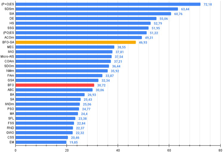
Figure 3. The histogram of algorithm test results (on a scale from 0 to 100, the more the better,

where 100 is the maximum possible theoretical result (the archive features a script for calculating the rating table)

BFO-GA pros and cons:

Advantages:

1. Algorithm high operation speed.
   
2. Simple implementation.
3. Good convergence on functions with a small number of parameters.
   

Disadvantages:

1. Low convergence on tasks with a large search space.
   

The article is accompanied by an archive with updated current versions of the algorithm codes described in previous articles. The author of the article is not responsible for the absolute accuracy in the description of canonical algorithms. Changes have been made to many of them to improve search capabilities. The conclusions and judgments presented in the articles are based on the results of the experiments.