Turtle Shell Evolution Algorithm (TSEA)
Contents
1. Introduction
2. Algorithm implementation
3.Test results
1. Introduction
The turtle is among the most ancient and amazing creations of nature. It wears a shell - a symbol of resilience, protection and survival. This majestic shield, formed throughout the turtle's life, embodies not only physical protection, but also symbolizes its continuous development and overcoming of obstacles.
The design on the shell is evidence of the uniqueness of its development path, symbolizing the harmony between time and the creature itself. The shell grows from a central point called the umbilical cord. New layers are added to the existing shell, resulting in the formation of different patterns. Each segment of the pattern represents a different year or season of the turtle's growth. Layer by layer, year after year, the shell matures along with the turtle. It takes on new patterns, forming unique clusters that are a reflection of the animal's life experiences and growth.
The turtle's shell consists of two main parts: the upper part called a carapace, and the lower part called a plastron. The growth of a turtle's shell occurs as a result of metamorphosis. The patterns on a turtle's shell are the result of a complex interaction of many factors, including genetics, environment, and the growth of the shell itself.
The turtle shell is composed of biological tissue and carbonate substances, such as calcium and magnesium. The carbonate structure of the shell provides it with strength and protects the turtle's internal organs. The shell of young turtles consists of soft cartilaginous plates, which harden and turn into bones over time. The shell grows due to the regular deposition of new layers of bone tissue under the turtle's skin. This process allows the shell to increase in size as the turtle grows and may result in new patterns appearing or existing ones changing over time.
The patterns on the turtle's shell are not random. They are formed as a result of certain biological processes and can be classified into different groups or "clusters" based on their shape, color and location. For example, some turtles have star-shaped patterns, while others have patterns that resemble leopard skin. As a turtle's shell grows, the patterns on it can change and evolve. This may result in a change in the cluster the pattern belongs to. For example, a pattern that was originally classified as "star" may become more complex over time.
It is important to note that each turtle has unique patterns on its shell, which help it adapt to its environment and perform important functions such as camouflage or attracting mates for breeding.
The patterns on the turtle shell inspired me to create an original optimization algorithm, and the evolution of the turtle shell became a metaphor for the process of merging and clustering data and determined the creation of a new tool that can adapt and evolve based on experience and knowledge.
2. Algorithm implementation
The idea behind the turtle shell evolution algorithm is to emulate the growth of the shell through the gradual formation of new keratinized areas of skin, which represent solutions to the optimization problem. In this model, the best solutions become harder and are located closer to the outer surface, while the less successful solutions remain softer and are located inside.
The shell in this context is divided into clusters that form a pattern on its surface, and its layers are simulated through vertical division into clusters. The process of emulating the growth of the shell in the algorithm includes movement both upward (outward) and downward (inward), as well as extension. A unique feature of this optimization algorithm is the preservation of less successful solutions, which is manifested in the growth of the shell inward. The inner layer of the shell is the only one that expands in both directions, while the other layers only expand outward, with the worst solutions being replaced by new ones. Each vertical cluster (layer) has a limited capacity for solutions; if the maximum number is not reached, solutions are simply added, otherwise the solution is replaced according to the described principle.
Figure 1 clearly shows the clustering of solutions according to their quality and the distance between them. For better understanding, a hypothetical example with a one-dimensional solution space is used. This diagram allows us to clearly see how clusters are formed depending on the quality and proximity of solutions to each other.
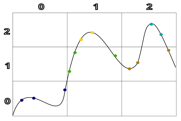
Figure 1. Clustering by solution quality and distance between solutions in the TSEA algorithm
Let's write a pseudocode for the TSEA algorithm:
1. Generate random individuals for the population.
2. Calculate FF.
3. Initial clustering of the population vertically.
4. Initial K-Means population clustering horizontally.
5. Place the population in a shell.
6. Generate a new population based on the data in the shell:
6.1. With the probability of 0.8:
Select a cluster vertically.
Select the best agent in the cell, or any random one in the cell with the probability of 0.5.
Use the selected agent in the cell, or use the best global solution with the probability of 0.6.
Create a new agent coordinate using the power distribution.
6.2 Or:
Select a cluster vertically.
Select two clusters vertically and randomly select an agent from them.
Create a new coordinate as the average value of the coordinates of the selected agents.
7. Calculate FF.
8. Population clustering vertically.
9. Define the belonging of agents to the clusters of the K-NN shell (the method of nearest N neighbors).
10. Perform vertical clustering of the shell every 50 epochs.
11. Place the population in a shell.
12. Repeat from p. 6.
Select the cluster vertically according to the quadratic law (Fig. 2), which determines the higher probability of being selected for the last (best) cluster on the list compared to the 0 th (worst) cluster.
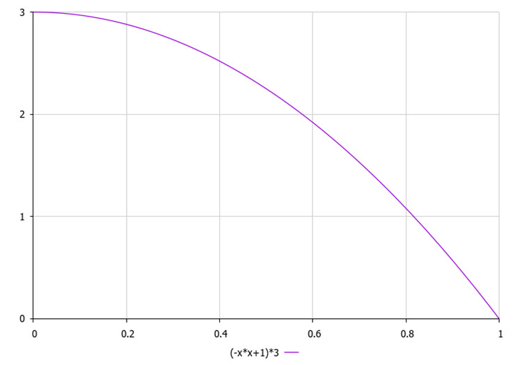
Figure 2. The law of probability of choosing a cluster vertically (by quality), where 3 is the number of clusters
Thus, the logic of creating new sections of the shell (agents - solutions to the optimization problem) is as follows:
- Selecting the shell layer (vertical cluster). The probability of choosing the top, harder layer is higher than the lower, less hard layers.
- Selecting carapace sections from horizontal clusters in the selected layer.
- "Fusing" the selected sections.
The probability of "fusing" (hardening) is higher for the upper layers than for the lower ones.
Now that we have the pseudocode and the law of agent selection in the parent population, the task is 99% complete. Of course, I am kidding. We still have to write the code.
We will describe the TSEA algorithm optimization agent as the S_TSEA_Agent structure. We will need cluster labels vertically and horizontally.
1. The structure contains the following fields:
- c[] - array for storing agent coordinates
- f - variable for storing the agent score (fitness)
- label - cluster membership label
- labelClustV - vertical clustering
- minDist - minimum distance to the nearest centroid
2. Init is a method of the S_TSEA_Agent structure that initializes the structure fields. It takes the "coords" integer argument used to resize the "c" array using the ArrayResize function.
3. f = -DBL_MAX - sets the initial value of the "f" variable equal to the minimum possible value of a 'double' number.
4. label = -1 and labelClustV = -1 - initialize cluster membership labels to -1.
5. minDist = DBL_MAX - sets the initial value of the "minDist" variable equal to the minimum possible value of a double number.
This code represents the basic data structure for agents in the TSEA optimization algorithm and initializes their fields when a new agent is created. This allows agents to store information about their current state and update it as the algorithm executes.
//——————————————————————————————————————————————————————————————————————————————
struct S_TSEA_Agent
{
    double c     [];     //coordinates
    double f;            //fitness
    int    label;        //cluster membership label
    int    labelClustV;  //clusters vertically
    double minDist;      //minimum distance to the nearest centroid

    void Init (int coords)
    {
      ArrayResize (c,     coords);
      f           = -DBL_MAX;
      label       = -1;
      labelClustV = -1;
      minDist     = DBL_MAX;
    }
};
//——————————————————————————————————————————————————————————————————————————————
We need to describe the turtle shell, which is a two-dimensional array, in which fitness clusters are arranged vertically and location clusters are arranged horizontally. Each cell of the two-dimensional array contains from 0 to the maximum value specified in the external parameters of the algorithm.
Describe the horizontal cluster with the S_TSEA_horizontal structure, which contains the fields:
- indBest - index of the best agent in the cell
- agent[] - array of S_TSEA_Agent structures used to store agents
We can describe the vertical cluster using the S_TSEA_horizontal structure containing the fields:
- cell[] - array of S_TSEA_horizontal structures.
Thus, the code gives us the ability to describe the turtle shell in two directions of a two-dimensional array. We can store optimization agents in each cell of the array. In essence, the shell is a specially structured parent population that will be convenient to access when creating child agents.
//——————————————————————————————————————————————————————————————————————————————
struct S_TSEA_horizontal
{
    int indBest;
    S_TSEA_Agent agent [];
};

struct S_TSEA_vertical
{
    S_TSEA_horizontal cell [];
};

//——————————————————————————————————————————————————————————————————————————————
To perform clustering, according to the given pseudocode, the TSEA algorithm applies two clustering methods: K-Means and K-NN. We already considered K-Means in the article about the BSO algorithm. Let's recall what the cluster structure looks like:
- centroid[] - array for storing the coordinates of the cell centroid
- f - variable for storing the score (fitness) of the centroid
- count - number of agents in the cluster
- agentList[] - list of agents in the cluster
- Init - method of the S_Cluster structure that initializes the structure fields
//——————————————————————————————————————————————————————————————————————————————
struct S_Cluster
{
    double centroid [];  //cluster centroid
    double f;            //centroid fitness
    int    count;        //number of points in the cluster

    void Init (int coords)
    {
      ArrayResize (centroid, coords);
      f     = -DBL_MAX;
      count = 0;
      ArrayResize (ideasList, 0, 100);
    }
};
//——————————————————————————————————————————————————————————————————————————————
To determine the belonging of a child agent to the corresponding cluster, we will use the K-NN method (the k-nearest neighbors method).
In addition to the K-Means method, the C_TSEA_clusters class contains the following methods:
1. VectorDistance method:
- The method calculates the Euclidean distance between "v1" and "v2" vectors represented by arrays of 'double' numbers.
- It uses the Euclidean distance equation:
 .
. - The calculated distance is returned.
2. DistanceIndex structure:
- The structure represents a pair of values: "distance" and "index".
- The structure is used to store distances from a point to other points and their indices.
3. BubbleSort method:
- The method sorts an array of objects of DistanceIndex type using the bubble sort method in distance ascending order.
- A temporary "temp" variable is used to exchange array elements.
4. The KNN method implements the k-nearest neighbors algorithm for classifying a "point":
- It calculates the distances from the "point" to all points in the "data" array, sorts these distances and determines whether the point belongs to one of the n_clusters - clusters based on k nearest neighbors.
- The "votes" array is used to calculate the votes of each cluster.
- The index of the cluster with the highest number of votes is returned.
//——————————————————————————————————————————————————————————————————————————————
class C_TSEA_clusters
{
  public:

  double VectorDistance (double &v1 [], double &v2 [])
  {
    double distance = 0.0;
    for (int i = 0; i < ArraySize (v1); i++)
    {
      distance += (v1 [i] - v2 [i]) * (v1 [i] - v2 [i]);
    }
    return MathSqrt (distance);
  }

  struct DistanceIndex
  {
      double distance;
      int index;
  };

  void BubbleSort (DistanceIndex &arr [], int start, int end)
  {
    for (int i = start; i < end; i++)
    {
      for (int j = start; j < end - i; j++)
      {
        if (arr [j].distance > arr [j + 1].distance)
        {
          DistanceIndex temp = arr [j];
          arr [j] = arr [j + 1];
          arr [j + 1] = temp;
        }
      }
    }
  }

  int KNN (S_TSEA_Agent &data [], S_TSEA_Agent &point, int k_neighbors, int n_clusters)
  {
    int n = ArraySize (data);
    DistanceIndex distances_indices [];

    // Calculate the distances from a point to all other points
    for (int i = 0; i < n; i++)
    {
      DistanceIndex dist;
      dist.distance = VectorDistance (point.c, data [i].c);
      dist.index = i;
      ArrayResize (distances_indices, n);
      distances_indices [i] = dist;
    }

    // Sort the distances
    BubbleSort (distances_indices, 0, n - 1);

    // Define the cluster for the point
    int votes [];
    ArrayResize (votes, n_clusters);
    ArrayInitialize (votes, 0);

    for (int j = 0; j < k_neighbors; j++)
    {
      int label = data [distances_indices [j].index].label;

      if (label != -1 && label < n_clusters)
      {
        votes [label]++;
      }
    }

    int max_votes = 0;
    int max_votes_cluster = -1;

    for (int j = 0; j < n_clusters; j++)
    {
      if (votes [j] > max_votes)
      {
        max_votes = votes [j];
        max_votes_cluster = j;
      }
    }

    return max_votes_cluster;
  }
};
//——————————————————————————————————————————————————————————————————————————————
Let's move on to the description of the C_AO_TSEA class derived from the C_AO base class. The class implements the "Turtle Shell Evolution Algorithm" (TSEA) algorithm. Class fields and methods:
1. C_AO_TSEA - the constructor initializes the class fields. It sets the name of the algorithm, its description and a link to the article about the algorithm. It also sets the algorithm parameters such as: population size, number of vertical and horizontal clusters, number of nearest neighbors and maximum number of agents in a cell.
2. SetParams - the method sets the algorithm parameters based on the values of the "params" array.
3. Init - the method initializes the algorithm. It accepts minimum and maximum search ranges, search step and number of epochs.
4. The Moving and Revision methods are the main methods of the TSEA algorithm, which implement its basic logic.
5. The vClusters, hClusters, neighbNumb and maxAgentsInCell fields are the algorithm parameters that are set in the constructor and can be changed using the SetParams method.
6. The agent, cell and clusters arrays are the data structures used by the algorithm. They contain information about agents, cells and clusters respectively.
7. The "km" object of the C_TSEA_clusters class is used to perform clustering operations.
8. The minFval, stepF, epochs and epochsNow private fields are internal variables. They are not intended to be accessed from outside the class.
//——————————————————————————————————————————————————————————————————————————————
class C_AO_TSEA : public C_AO
{
  public: //--------------------------------------------------------------------
  ~C_AO_TSEA () { }
  C_AO_TSEA ()
  {
    ao_name = "TSEA";
    ao_desc = "Turtle Shell Evolution Algorithm";
    ao_link = "https://www.mql5.com/ru/articles/14789";

    popSize         = 100; //population size

    vClusters       = 3;   //number of vertical clusters
    hClusters       = 10;  //number of horizontal clusters
    neighbNumb      = 5;   //number of nearest neighbors
    maxAgentsInCell = 3;   //max agents in cell

    ArrayResize (params, 5);

    params [0].name = "popSize";          params [0].val  = popSize;

    params [1].name = "vClusters";        params [1].val  = vClusters;
    params [2].name = "hClusters";        params [2].val  = hClusters;
    params [3].name = "neighbNumb";       params [3].val  = neighbNumb;
    params [4].name = "maxAgentsInCell";  params [4].val  = maxAgentsInCell;
  }

  void SetParams ()
  {
    popSize         = (int)params [0].val;

    vClusters       = (int)params [1].val;
    hClusters       = (int)params [2].val;
    neighbNumb      = (int)params [3].val;
    maxAgentsInCell = (int)params [4].val;
  }

  bool Init (const double &rangeMinP  [], //minimum search range
             const double &rangeMaxP  [], //maximum search range
             const double &rangeStepP [], //step search
             const int     epochsP = 0);  //number of epochs

  void Moving    ();
  void Revision  ();
  void Injection (const int popPos, const int coordPos, const double value);

  //----------------------------------------------------------------------------
  int    vClusters;      //number of vertical clusters
  int    hClusters;      //number of horizontal clusters
  int    neighbNumb;     //number of nearest neighbors
  int    maxAgentsInCell;

  S_TSEA_Agent    agent   [];
  S_TSEA_vertical cell    [];

  S_Cluster      clusters [];
  C_TSEA_clusters km;

  private: //-------------------------------------------------------------------
  double minFval;
  double stepF;

  int    epochs;
  int    epochsNow;
};
//——————————————————————————————————————————————————————————————————————————————
The Init method of the C_AO_TSEA class initializes the TSEA algorithm. Detailed description of its work is provided below:
1. StandardInit (rangeMinP, rangeMaxP, rangeStepP) - the method is called for standard initialization of the algorithm. It accepts minimum and maximum search ranges and search step. If initialization fails, the method returns 'false'.
2. ArrayResize (agent, popSize) resizes the "agent" array to the "popSize" population size. The Init(coords) method is then called for each agent to initialize it.
3. ArrayResize (clusters, hClusters) resizes the "clusters" array to the number of hClusters horizontal clusters. The Init(coords) method is called next for each cluster to initialize it.
4. ArrayResize (cell, vClusters) resizes the "cell" array to the number of vClusters vertical clusters. The cell[i].cell array and the array of agents in each cell are then initialized for each cell.
5. "minFval = DBL_MAX", "stepF = 0.0", "epochs = epochsP", "epochsNow = 0". Initializing the algorithm internal variables.
6. At the end, the method returns 'true' indicating that the initialization was successful.
//——————————————————————————————————————————————————————————————————————————————
bool C_AO_TSEA::Init (const double &rangeMinP  [], //minimum search range
                      const double &rangeMaxP  [], //maximum search range
                      const double &rangeStepP [], //step search
                      const int     epochsP = 0)   //number of epochs
{
  if (!StandardInit (rangeMinP, rangeMaxP, rangeStepP)) return false;

  //----------------------------------------------------------------------------
  ArrayResize (agent, popSize);
  for (int i = 0; i < popSize; i++) agent [i].Init (coords);

  ArrayResize (clusters, hClusters);
  for (int i = 0; i < hClusters; i++) clusters [i].Init (coords);

  ArrayResize (cell, vClusters);

  for (int i = 0; i < vClusters; i++)
  {
    ArrayResize (cell [i].cell, hClusters);

    for (int c = 0; c < hClusters; c++) ArrayResize (cell [i].cell [c].agent, 0, maxAgentsInCell);
  }

  minFval   = DBL_MAX;
  stepF     = 0.0;
  epochs    = epochsP;
  epochsNow = 0;

  return true;
}
//——————————————————————————————————————————————————————————————————————————————
The Moving method of the C_AO_TSEA class implements the basic logic of agent movement in the TSEA algorithm. Brief description of the main steps:
1. Population initialization:
- If this is the first iteration (revision == false), random individuals are generated into the population.
- Otherwise, the population is updated based on existing decisions.
2. Updating the population:
- The best solution is found for each cluster (vClusters х hClusters).
- New solutions are formed as follows:
- The best solution is copied from a random cluster with some bias with the probability of 0.5
- With the probability of 0.2, a new solution is formed as the average between two random solutions from different clusters
- New solution coordinates are generated using a power-law distribution to maintain proximity to the best solutions.
3. Updating agents (individuals) in the population
This method implements the basic idea of the turtle shell evolution, where the best solutions become "harder" and are located closer to the outer surface, while the less successful solutions remain "softer" and are located inside. Clustering of solutions and retention of less successful variants ensures the algorithm flexibility and adaptability.
//——————————————————————————————————————————————————————————————————————————————
void C_AO_TSEA::Moving ()
{
  epochsNow++;

  //----------------------------------------------------------------------------
  //1. Generate random individuals for the population
  if (!revision)
  {
    for (int i = 0; i < popSize; i++)
    {
      for (int c = 0; c < coords; c++)
      {
        a [i].c [c] = u.RNDfromCI (rangeMin [c], rangeMax [c]);
        a [i].c [c] = u.SeInDiSp  (a [i].c [c], rangeMin [c], rangeMax [c], rangeStep [c]);

        agent [i].c [c] = a [i].c [c];
      }
    }

    return;
  }

  //----------------------------------------------------------------------------
  int    vPos = 0;
  int    hPos = 0;
  int    pos  = 0;
  int    size = 0;
  double val  = 0.0;
  double rnd  = 0.0;
  double min  = 0.0;
  double max  = 0.0;

  for (int v = 0; v < vClusters; v++)
  {
    for (int h = 0; h < hClusters; h++)
    {
      size = ArraySize (cell [v].cell [h].agent);

      if (size > 0)
      {
        max = -DBL_MAX;
        pos = -1;

        for (int c = 0; c < size; c++)
        {
          if (cell [v].cell [h].agent [c].f > max)
          {
            max = cell [v].cell [h].agent [c].f;
            pos = c;
            cell [v].cell [h].indBest = c;
          }
        }
      }
    }
  }

  for (int i = 0; i < popSize; i++)
  {
    if (u.RNDprobab () < 0.8)
    {
      while (true)
      {
        rnd = u.RNDprobab ();
        rnd = (-rnd * rnd + 1.0) * vClusters;

        vPos = (int)rnd;
        if (vPos > vClusters - 1) vPos = vClusters - 1;

        hPos = u.RNDminusOne (hClusters);

        size = ArraySize (cell [vPos].cell [hPos].agent);

        if (size > 0) break;
      }

      pos = u.RNDminusOne (size);

      if (u.RNDprobab () < 0.5) pos = cell [vPos].cell [hPos].indBest;

      for (int c = 0; c < coords; c++)
      {
        if (u.RNDprobab () < 0.6) val = cell [vPos].cell [hPos].agent [pos].c [c];
        else                      val = cB [c];

        double dist = (rangeMax [c] - rangeMin [c]) * 0.1;
        min = val - dist; if (min < rangeMin [c]) min = rangeMin [c];
        max = val + dist; if (max > rangeMax [c]) max = rangeMax [c];

        val = u.PowerDistribution (val, min, max, 30);

        a [i].c [c] = u.SeInDiSp  (val, rangeMin [c], rangeMax [c], rangeStep [c]);

        agent [i].c [c] = a [i].c [c];
      }
    }
    else
    {
      int size2 = 0;
      int hPos2 = 0;
      int pos2  = 0;

      while (true)
      {
        rnd = u.RNDprobab ();
        rnd = (-rnd * rnd + 1.0) * vClusters;

        vPos = (int)rnd;
        if (vPos > vClusters - 1) vPos = vClusters - 1;

        hPos = u.RNDminusOne (hClusters);
        size = ArraySize (cell [vPos].cell [hPos].agent);

        hPos2 = u.RNDminusOne (hClusters);
        size2 = ArraySize (cell [vPos].cell [hPos2].agent);

        if (size > 0 && size2 > 0) break;
      }

      pos  = u.RNDminusOne (size);
      pos2 = u.RNDminusOne (size2);

      for (int c = 0; c < coords; c++)
      {
        val = (cell [vPos].cell [hPos ].agent [pos ].c [c] +
               cell [vPos].cell [hPos2].agent [pos2].c [c]) * 0.5;

        a [i].c [c] = u.SeInDiSp  (val, rangeMin [c], rangeMax [c], rangeStep [c]);

        agent [i].c [c] = a [i].c [c];
      }
    }
  }
}
//——————————————————————————————————————————————————————————————————————————————
The Revision method of the C_AO_TSEA class implements the stage of redistribution of the turtle shell sections in the TSEA algorithm.
It is responsible for revising (updating) the agent population and updating the best global solution.
The main steps of this part of the algorithm are:
2. Labeling agents into vertical "labelClustV" clusters based on their fitness.
3. If this is the first iteration (revision == false), then the clustering of agents is initialized using the K-Means algorithm.
4. If this is not the first iteration, then the following is performed:
- All agents are collected into the single 'data' array.
- For each agent in the population, its horizontal "label" cluster is determined using the K-Nearest Neighbors algorithm.
- The "cell" structure, storing agents divided into clusters, is updated every 50 epochs.
5. Placing each agent in the appropriate cell. If the cell is already filled, the agent replaces the one with the lowest (or highest, if the cell is at the bottom level) fitness in the cell.
The main idea of this stage is to maintain the structure of the shell, where the best solutions are located closer to the outer surface, while the less successful ones are located inside. Clustering of agents and dynamic updating of the shell structure ensure the algorithm flexibility and adaptability.
//——————————————————————————————————————————————————————————————————————————————
void C_AO_TSEA::Revision ()
{
  //get fitness--------------------------------------------------
  int pos = -1;

  for (int i = 0; i < popSize; i++)
  {
    agent [i].f = a [i].f;

    if (a [i].f > fB)
    {
      fB = a [i].f;
      pos = i;
    }

    if (a [i].f < minFval) minFval = a [i].f;
  }

  if (pos != -1) ArrayCopy (cB, a [pos].c, 0, 0, WHOLE_ARRAY);

  stepF = (fB - minFval) / vClusters;

  //Vertical layout of the child population-----------------------------------
  for (int i = 0; i < popSize; i++)
  {
    if (agent [i].f == fB) agent [i].labelClustV = vClusters - 1;
    else
    {
      agent [i].labelClustV = int((agent [i].f - minFval) / stepF);
      if (agent [i].labelClustV > vClusters - 1) agent [i].labelClustV = vClusters - 1;
    }
  }

  //----------------------------------------------------------------------------
  if (!revision)
  {
    km.KMeansPlusPlusInit (agent, popSize, clusters);
    km.KMeans             (agent, popSize, clusters);

    revision = true;
  }
  //----------------------------------------------------------------------------
  else
  {
    static S_TSEA_Agent data [];
    ArrayResize (data, 0, 1000);
    int size = 0;

    for (int v = 0; v < vClusters; v++)
    {
      for (int h = 0; h < hClusters; h++)
      {
        for (int c = 0; c < ArraySize (cell [v].cell [h].agent); c++)
        {
          size++;
          ArrayResize (data, size);

          data [size - 1] = cell [v].cell [h].agent [c];
        }
      }
    }

    for (int i = 0; i < popSize; i++)
    {
      agent [i].label = km.KNN (data, agent [i], neighbNumb, hClusters);
    }

    if (epochsNow % 50 == 0)
    {
      for (int v = 0; v < vClusters; v++)
      {
        for (int h = 0; h < hClusters; h++)
        {
          ArrayResize (cell [v].cell [h].agent, 0);
        }
      }

      for (int i = 0; i < ArraySize (data); i++)
      {
        if (data [i].f == fB) data [i].labelClustV = vClusters - 1;
        else
        {
          data [i].labelClustV = int((data [i].f - minFval) / stepF);
          if (data [i].labelClustV > vClusters - 1) data [i].labelClustV = vClusters - 1;
        }

        int v = data [i].labelClustV;
        int h = data [i].label;

        int size = ArraySize (cell [v].cell [h].agent) + 1;
        ArrayResize (cell [v].cell [h].agent, size);

        cell [v].cell [h].agent [size - 1] = data [i];
      }
    }
  }

  //Place the population in the shell------------------------------------
  for (int i = 0; i < popSize; i++)
  {
    int v = agent [i].labelClustV;
    int h = agent [i].label;

    int size = ArraySize (cell [v].cell [h].agent);
    int pos    = 0;
    int posMin = 0;
    int posMax = 0;

    if (size >= maxAgentsInCell)
    {
      double minF =  DBL_MAX;
      double maxF = -DBL_MAX;

      for (int c = 0; c < maxAgentsInCell; c++)
      {
        if (cell [v].cell [h].agent [c].f < minF)
        {
          minF = cell [v].cell [h].agent [c].f;
          posMin = c;
        }
        if (cell [v].cell [h].agent [c].f > maxF)
        {
          maxF = cell [v].cell [h].agent [c].f;
          posMax = c;
        }
      }

      if (v == 0)
      {
        if (agent [i].f < minF)
        {
          pos = posMin;
        }
        else
        {
          pos = posMax;
        }
      }
      else  pos = posMin;
    }
    else
    {
      ArrayResize (cell [v].cell [h].agent, size + 1);
      pos = size;
    }

    cell [v].cell [h].agent [pos] = agent [i];
  }
}
//——————————————————————————————————————————————————————————————————————————————
3. Test results
TSEA results:
TSEA|Turtle Shell Evolution Algorithm|100.0|3.0|10.0|5.0|3.0|
=============================
5 Hilly's; Func runs: 10000; result: 0.811921100517765
25 Hilly's; Func runs: 10000; result: 0.5537631430428238
500 Hilly's; Func runs: 10000; result: 0.2813575513298344
=============================
5 Forest's; Func runs: 10000; result: 0.9564485273109922
25 Forest's; Func runs: 10000; result: 0.481362270824773
500 Forest's; Func runs: 10000; result: 0.181400891410298
=============================
5 Megacity's; Func runs: 10000; result: 0.6676923076923076
25 Megacity's; Func runs: 10000; result: 0.3633846153846153
500 Megacity's; Func runs: 10000; result: 0.11670769230769343
=============================
All score: 4.41404 (49.04%)
The total score for all test functions is 4.41404, which corresponds to 49.04% of the theoretical optimal solution.
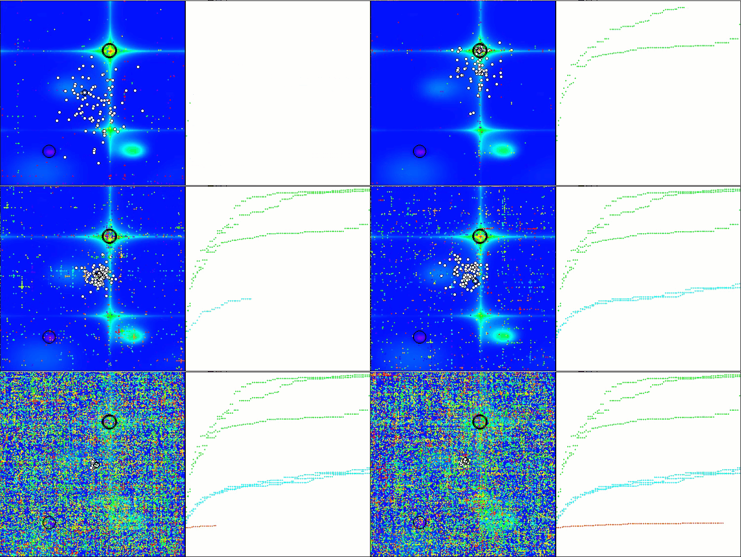
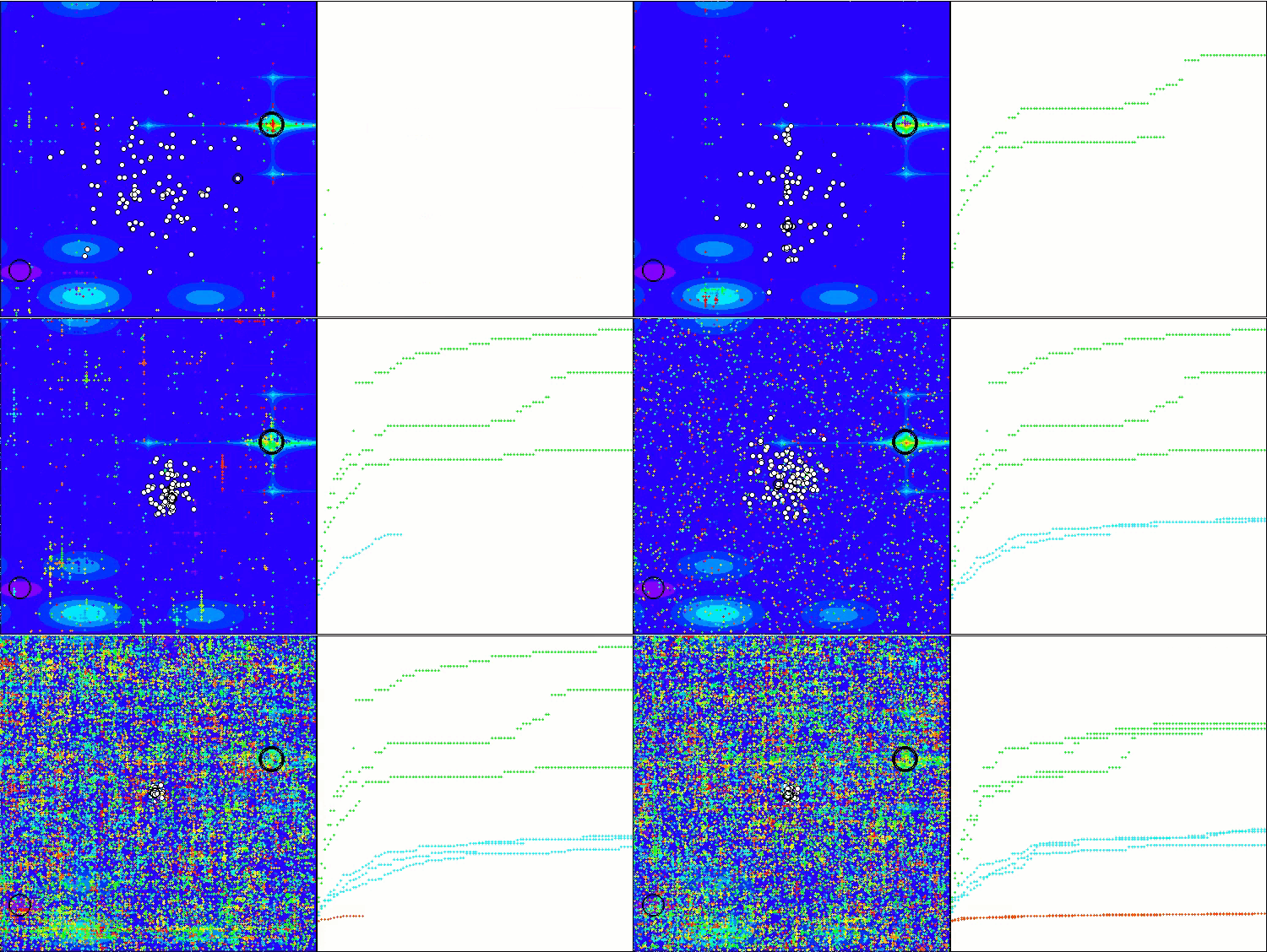
Visualization of the test bench operation demonstrates good convergence of the algorithm. For all test functions, there is a scatter of trajectories on the convergence graph. However, with an increase in the degrees of freedom, this scatter decreases. The use of clustering in the algorithm, as well as maintaining a constant number of agents in each cell, allows the algorithm to effectively explore significant areas of the fitness function.
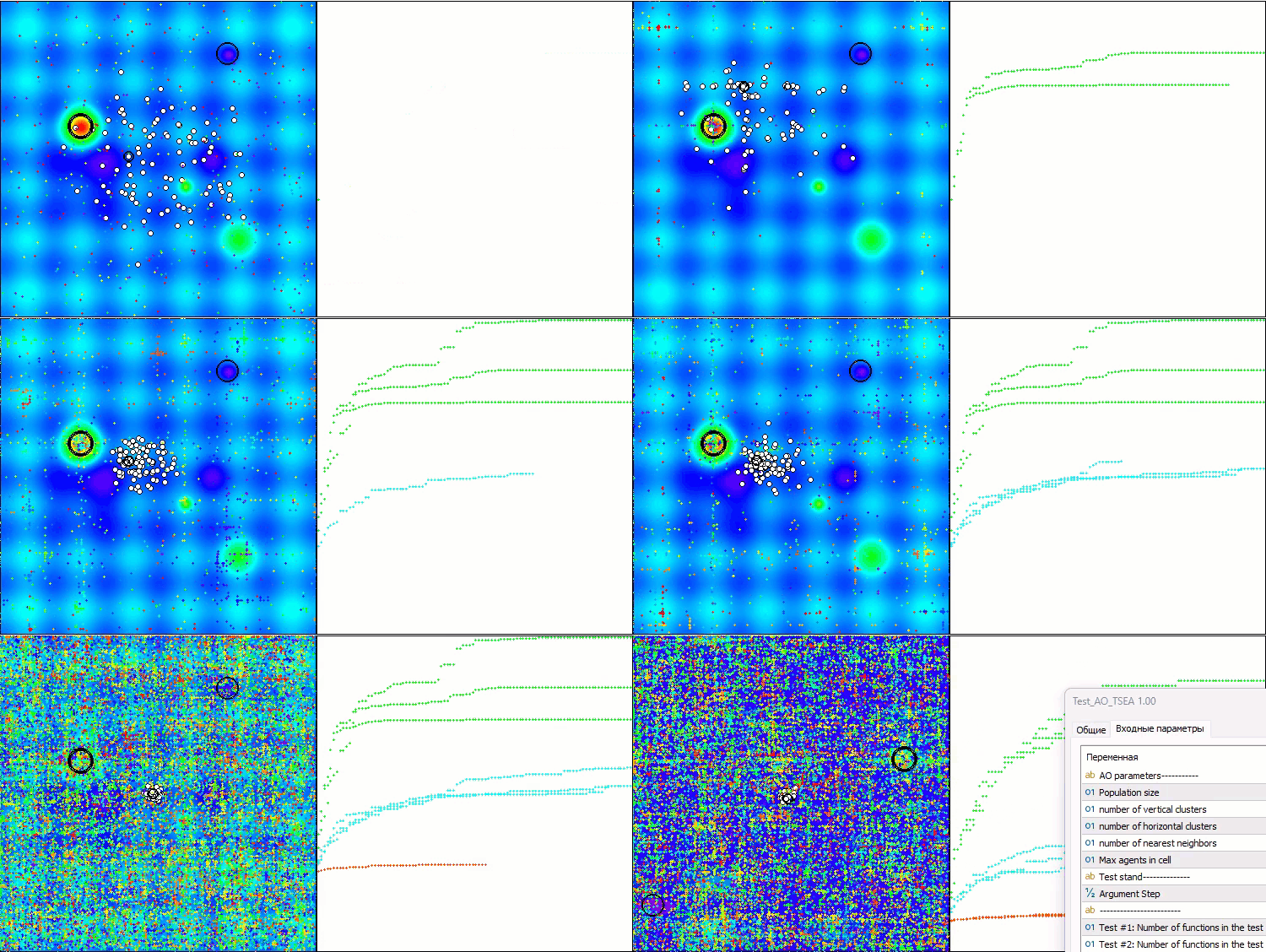
TSEA on the Hilly test function
TSEA on the Forest test function
TSEA on the Megacity test function
After checking on the test functions, the algorithm occupies a worthy 6th place at the top of the final rating table.
# | AO | Description | Hilly | Hilly final | Forest | Forest final | Megacity (discrete) | Megacity final | Final result | % of MAX | ||||||
| 10 p (5 F) | 50 p (25 F) | 1000 p (500 F) | 10 p (5 F) | 50 p (25 F) | 1000 p (500 F) | 10 p (5 F) | 50 p (25 F) | 1000 p (500 F) | ||||||||
| 1 | BGA | binary genetic algorithm | 0.99992 | 0.99484 | 0.50483 | 2.49959 | 1.00000 | 0.99975 | 0.32054 | 2.32029 | 0.90667 | 0.96400 | 0.23035 | 2.10102 | 6.921 | 76.90 |
| 2 | (P+O)ES | (P+O) evolution strategies | 0.99934 | 0.91895 | 0.56297 | 2.48127 | 1.00000 | 0.93522 | 0.39179 | 2.32701 | 0.83167 | 0.64433 | 0.21155 | 1.68755 | 6.496 | 72.18 |
| 3 | SDSm | stochastic diffusion search M | 0.93066 | 0.85445 | 0.39476 | 2.17988 | 0.99983 | 0.89244 | 0.19619 | 2.08846 | 0.72333 | 0.61100 | 0.10670 | 1.44103 | 5.709 | 63.44 |
| 4 | ESG | evolution of social groups | 0.99906 | 0.79654 | 0.35056 | 2.14616 | 1.00000 | 0.82863 | 0.13102 | 1.95965 | 0.82333 | 0.55300 | 0.04725 | 1.42358 | 5.529 | 61.44 |
| 5 | SIA | simulated isotropic annealing | 0.95784 | 0.84264 | 0.41465 | 2.21513 | 0.98239 | 0.79586 | 0.20507 | 1.98332 | 0.68667 | 0.49300 | 0.09053 | 1.27020 | 5.469 | 60.76 |
| 6 | TSEA | turtle shell evolution algorithm | 0.96798 | 0.64480 | 0.29672 | 1.90949 | 0.99449 | 0.61981 | 0.22708 | 1.84139 | 0.69077 | 0.42646 | 0.13598 | 1.25322 | 5.004 | 55.60 |
| 7 | DE | differential evolution | 0.95044 | 0.61674 | 0.30308 | 1.87026 | 0.95317 | 0.78896 | 0.16652 | 1.90865 | 0.78667 | 0.36033 | 0.02953 | 1.17653 | 4.955 | 55.06 |
| 8 | BSA | bird swarm algorithm | 0.90857 | 0.73661 | 0.25767 | 1.90285 | 0.90437 | 0.81619 | 0.16401 | 1.88457 | 0.61692 | 0.54154 | 0.10951 | 1.26797 | 5.055 | 56.17 |
| 9 | HS | harmony search | 0.86509 | 0.68782 | 0.32527 | 1.87818 | 0.99999 | 0.68002 | 0.09590 | 1.77592 | 0.62000 | 0.42267 | 0.05458 | 1.09725 | 4.751 | 52.79 |
| 10 | SSG | saplings sowing and growing | 0.77839 | 0.64925 | 0.39543 | 1.82308 | 0.85973 | 0.62467 | 0.17429 | 1.65869 | 0.64667 | 0.44133 | 0.10598 | 1.19398 | 4.676 | 51.95 |
| 11 | (PO)ES | (PO) evolution strategies | 0.79025 | 0.62647 | 0.42935 | 1.84606 | 0.87616 | 0.60943 | 0.19591 | 1.68151 | 0.59000 | 0.37933 | 0.11322 | 1.08255 | 4.610 | 51.22 |
| 12 | BSO | brain storm optimization | 0.91301 | 0.56222 | 0.30047 | 1.77570 | 0.97162 | 0.57162 | 0.23449 | 1,77772 | 0.60462 | 0.27138 | 0.12011 | 0.99611 | 4.550 | 50.55 |
| 13 | WOAm | wale optimization algorithm M | 0.84521 | 0.56298 | 0.26263 | 1.67081 | 0.93100 | 0.52278 | 0.16365 | 1.61743 | 0.66308 | 0.41138 | 0.11357 | 1.18803 | 4.476 | 49.74 |
| 14 | ACOm | ant colony optimization M | 0.88190 | 0.66127 | 0.30377 | 1.84693 | 0.85873 | 0.58680 | 0.15051 | 1.59604 | 0.59667 | 0.37333 | 0.02472 | 0.99472 | 4.438 | 49.31 |
| 15 | BFO-GA | bacterial foraging optimization - ga | 0.89150 | 0.55111 | 0.31529 | 1.75790 | 0.96982 | 0.39612 | 0.06305 | 1.42899 | 0.72667 | 0.27500 | 0.03525 | 1.03692 | 4.224 | 46.93 |
| 16 | MEC | mind evolutionary computation | 0.69533 | 0.53376 | 0.32661 | 1.55569 | 0.72464 | 0.33036 | 0.07198 | 1.12698 | 0.52500 | 0.22000 | 0.04198 | 0.78698 | 3.470 | 38.55 |
| 17 | IWO | invasive weed optimization | 0.72679 | 0.52256 | 0.33123 | 1.58058 | 0.70756 | 0.33955 | 0.07484 | 1.12196 | 0.42333 | 0.23067 | 0.04617 | 0.70017 | 3.403 | 37.81 |
| 18 | Micro-AIS | micro artificial immune system | 0.79547 | 0.51922 | 0.30861 | 1.62330 | 0.72956 | 0.36879 | 0.09398 | 1.19233 | 0.37667 | 0.15867 | 0.02802 | 0.56335 | 3.379 | 37.54 |
| 19 | COAm | cuckoo optimization algorithm M | 0.75820 | 0.48652 | 0.31369 | 1.55841 | 0.74054 | 0.28051 | 0.05599 | 1.07704 | 0.50500 | 0.17467 | 0.03380 | 0.71347 | 3.349 | 37.21 |
| 20 | SDOm | spiral dynamics optimization M | 0.74601 | 0.44623 | 0.29687 | 1.48912 | 0.70204 | 0.34678 | 0.10944 | 1.15826 | 0.42833 | 0.16767 | 0.03663 | 0.63263 | 3.280 | 36.44 |
| 21 | NMm | Nelder-Mead method M | 0.73807 | 0.50598 | 0.31342 | 1.55747 | 0.63674 | 0.28302 | 0.08221 | 1.00197 | 0.44667 | 0.18667 | 0.04028 | 0.67362 | 3.233 | 35.92 |
| 22 | FAm | firefly algorithm M | 0.58634 | 0.47228 | 0.32276 | 1.38138 | 0.68467 | 0.37439 | 0.10908 | 1.16814 | 0.28667 | 0.16467 | 0.04722 | 0.49855 | 3.048 | 33.87 |
| 23 | GSA | gravitational search algorithm | 0.64757 | 0.49197 | 0.30062 | 1.44016 | 0.53962 | 0.36353 | 0.09945 | 1.00260 | 0.32667 | 0.12200 | 0.01917 | 0.46783 | 2.911 | 32.34 |
| 24 | BFO | bacterial foraging optimization | 0.61171 | 0.43270 | 0.31318 | 1.35759 | 0.54410 | 0.21511 | 0.05676 | 0.81597 | 0.42167 | 0.13800 | 0.03195 | 0.59162 | 2.765 | 30.72 |
| 25 | ABC | artificial bee colony | 0.63377 | 0.42402 | 0.30892 | 1.36671 | 0.55103 | 0.21874 | 0.05623 | 0.82600 | 0.34000 | 0.14200 | 0.03102 | 0.51302 | 2.706 | 30.06 |
| 26 | BA | bat algorithm | 0.59761 | 0.45911 | 0.35242 | 1.40915 | 0.40321 | 0.19313 | 0.07175 | 0.66810 | 0.21000 | 0.10100 | 0.03517 | 0.34617 | 2.423 | 26.93 |
| 27 | SA | simulated annealing | 0.55787 | 0.42177 | 0.31549 | 1.29513 | 0.34998 | 0.15259 | 0.05023 | 0.55280 | 0.31167 | 0.10033 | 0.02883 | 0.44083 | 2.289 | 25.43 |
| 28 | IWDm | intelligent water drops M | 0.54501 | 0.37897 | 0.30124 | 1.22522 | 0.46104 | 0.14704 | 0.04369 | 0.65177 | 0.25833 | 0.09700 | 0.02308 | 0.37842 | 2.255 | 25.06 |
| 29 | PSO | particle swarm optimisation | 0.59726 | 0.36923 | 0.29928 | 1.26577 | 0.37237 | 0.16324 | 0.07010 | 0.60572 | 0.25667 | 0.08000 | 0.02157 | 0.35823 | 2.230 | 24.77 |
| 30 | Boids | boids algorithm | 0.43340 | 0.30581 | 0.25425 | 0.99346 | 0.35718 | 0.20160 | 0.15708 | 0.71586 | 0.27846 | 0.14277 | 0.09834 | 0.51957 | 2.229 | 24.77 |
| 31 | MA | monkey algorithm | 0.59107 | 0.42681 | 0.31816 | 1.33604 | 0.31138 | 0.14069 | 0.06612 | 0.51819 | 0.22833 | 0.08567 | 0.02790 | 0.34190 | 2.196 | 24.40 |
| 32 | SFL | shuffled frog-leaping | 0.53925 | 0.35816 | 0.29809 | 1.19551 | 0.37141 | 0.11427 | 0.04051 | 0.52618 | 0.27167 | 0.08667 | 0.02402 | 0.38235 | 2.104 | 23.38 |
| 33 | FSS | fish school search | 0.55669 | 0.39992 | 0.31172 | 1.26833 | 0.31009 | 0.11889 | 0.04569 | 0.47467 | 0.21167 | 0.07633 | 0.02488 | 0.31288 | 2.056 | 22.84 |
| 34 | RND | random | 0.52033 | 0.36068 | 0.30133 | 1.18234 | 0.31335 | 0.11787 | 0.04354 | 0.47476 | 0.25333 | 0.07933 | 0.02382 | 0.35648 | 2.014 | 22.37 |
| 35 | GWO | grey wolf optimizer | 0.59169 | 0.36561 | 0.29595 | 1.25326 | 0.24499 | 0.09047 | 0.03612 | 0.37158 | 0.27667 | 0.08567 | 0.02170 | 0.38403 | 2.009 | 22.32 |
| 36 | CSS | charged system search | 0.44252 | 0.35454 | 0.35201 | 1.14907 | 0.24140 | 0.11345 | 0.06814 | 0.42299 | 0.18333 | 0.06300 | 0.02322 | 0.26955 | 1.842 | 20.46 |
| 37 | EM | electroMagnetism-like algorithm | 0.46250 | 0.34594 | 0.32285 | 1.13129 | 0.21245 | 0.09783 | 0.10057 | 0.41085 | 0.15667 | 0.06033 | 0.02712 | 0.24412 | 1.786 | 19.85 |
Summary
The idea of an optimization algorithm based on the growth of a turtle's shell turned out to be quite interesting. Even such slow animals can serve as inspiration and an example of "technical" solutions provided by nature in huge amounts. Based on the TSEA (Turtle Shell Evolution Algorithm) tests, we managed to define main features of the algorithm.
Preserving less successful solutions is a unique feature of the algorithm. This is evident in the fact that less successful variants are preserved in the inner layer of the shell. This approach allows maintaining diversity in the population and preventing premature convergence to local optima. It is important to remember that a local minimum that appears to be the worst solution may be close to the global optimum, so continuing to explore its vicinity makes sense. Although the algorithm may explore such areas less intensively than more promising locations, they still remain a focus of attention.
Dividing solutions into clusters vertically, simulating the layers of the shell, and horizontally, simulating the characteristic patterns on the surface, allows us to quite efficiently isolate areas of the solution space and study them separately. At the same time, the pattern on the shell remains mobile and can change and adapt to the surface of the fitness function.
The use of layering of the shell allows for the formation of new solutions within each layer. The upper hard layers do not interact with the lower soft layers, and vice versa. This is similar to the process of shell growth in a living turtle, but with the difference that the hard section from the lower layer can move to the upper layers due to periodic reclustering. This can be compared to shedding the old shell and forming a new one, which is stronger and better.
The algorithm demonstrates good performance on problems with different numbers of dimensions (scalability), which indicates its flexibility.
Overall, TSEA is an interesting approach that combines evolutionary algorithms and clustering mechanisms. However, I am confident that the algorithm potential is far from exhausted. At this point, only a few of the many different ways of creating new solutions have been used from the vast variety that were previously discussed in the articles. The algorithm remains in my focus and is open to further improvement. Perhaps, it will serve as a basis for some new modifications, similar to what happened with PSO and other well-known algorithms.
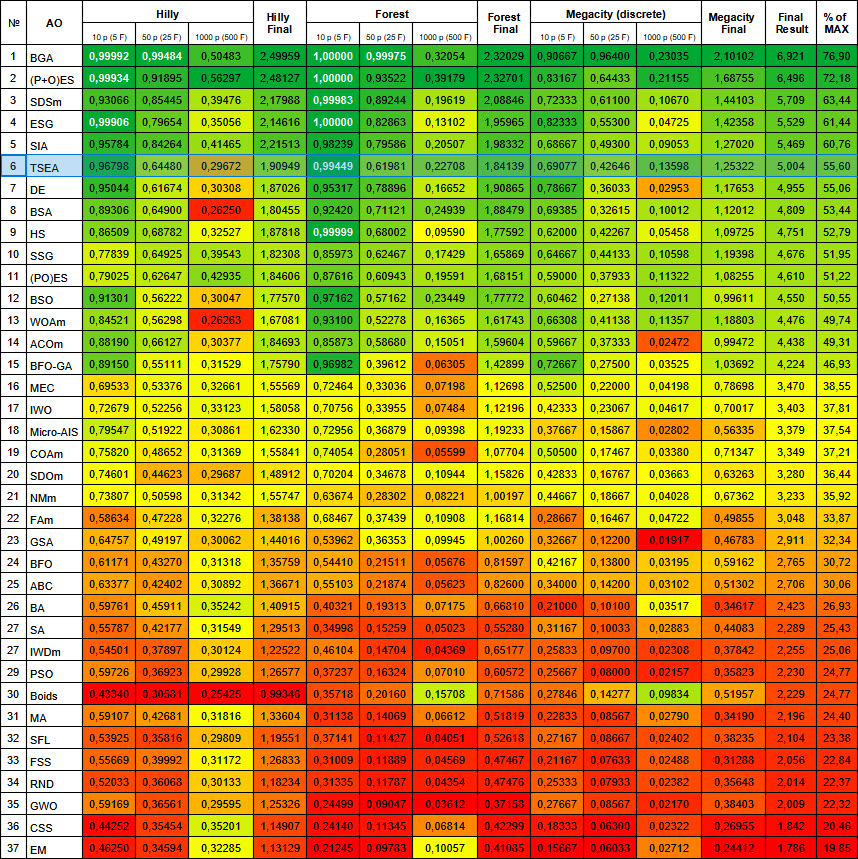
Figure 3. Color gradation of algorithms according to relevant tests Results greater than or equal to 0.99 are highlighted in white
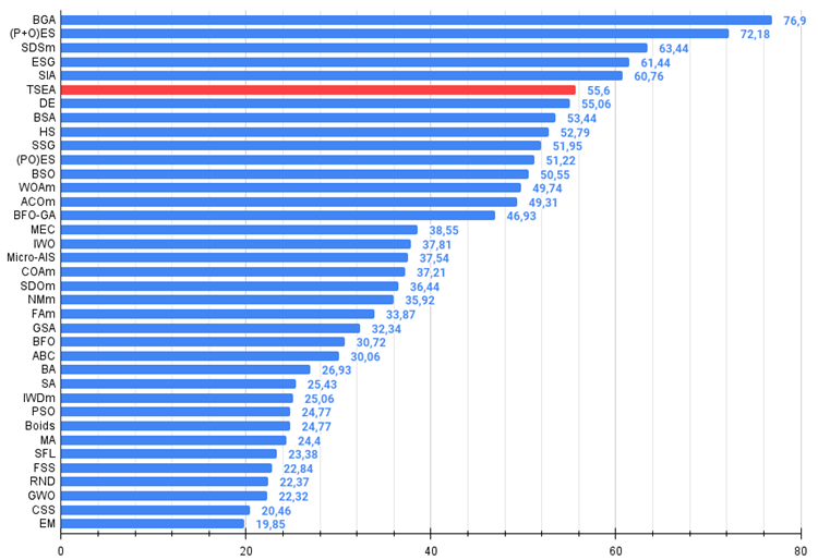
Figure 4. The histogram of algorithm test results (on a scale from 0 to 100, the more the better,
where 100 is the maximum possible theoretical result, the archive features a script for calculating the rating table)
TSEA pros and cons:
Advantages:
- Good convergence on various types of functions
- Small number of external parameters
Disadvantages:
- High scatter of results on low-dimensional functions
- High load on computing resources
The article is accompanied by an archive with the current versions of the algorithm codes. The author of the article is not responsible for the absolute accuracy in the description of canonical algorithms. Changes have been made to many of them to improve search capabilities. The conclusions and judgments presented in the articles are based on the results of the experiments.
github: https://github.com/JQSakaJoo/Population-optimization-algorithms-MQL5
CodeBase: https://www.mql5.com/ru/code/49355
Translated from Russian by MetaQuotes Ltd.
Original article: https://www.mql5.com/ru/articles/14789
Warning: All rights to these materials are reserved by MetaQuotes Ltd. Copying or reprinting of these materials in whole or in part is prohibited.
This article was written by a user of the site and reflects their personal views. MetaQuotes Ltd is not responsible for the accuracy of the information presented, nor for any consequences resulting from the use of the solutions, strategies or recommendations described.
 Using PSAR, Heiken Ashi, and Deep Learning Together for Trading
 Example of CNA (Causality Network Analysis), SMOC (Stochastic Model Optimal Control) and Nash Game Theory with Deep Learning
 MQL5 Wizard Techniques you should know (Part 39): Relative Strength Index
 Creating a Trading Administrator Panel in MQL5 (Part III): Enhancing the GUI with Visual Styling (I)
- Free trading apps
- Over 8,000 signals for copying
- Economic news for exploring financial markets
You agree to website policy and terms of use