Population optimization algorithms: Gravitational Search Algorithm (GSA)

Contents

1. Introduction
2. Algorithm
3. Test results

1. Introduction

Gravitational Search Algorithm (GSA) was proposed by E. Rashedi to solve the optimization problem, especially non-linear problems, following the principles of Newton's law of gravitation. In the proposed algorithm, particles are considered as objects and their performance is estimated taking into account their masses. Gravity is the tendency of masses to accelerate towards each other. It is one of the four fundamental forces in nature (the others are the electromagnetic force, the weak nuclear force and the strong nuclear force).

Every particle in the universe attracts every other particle. Gravity exists everywhere. Although it is the weakest force, it is the most visible one. Due to the gravitational force, people can walk on the Earth and planets can orbit the Sun. The gravitational force of any object is proportional to its mass. Thus, objects with more mass have more gravity. The inevitability of gravity distinguishes it from all other forces of nature. The way Newton's gravitational force behaves is called action at a distance. It is a general physical law deduced from empirical observation by what Isaac Newton called inductive reasoning. It is part of classical mechanics formulated in Newton's Philosophiae Naturalis Principia Mathematica (Principia) first published on July 5, 1687.

When in April 1686 Newton presented the first unpublished book to the Royal Society, Robert Hooke claimed that Newton received the inverse square law from him. In today's language, the law says that every point mass attracts every other point mass by a force acting along a line that intersects two points.

2. Algorithm

The article presents an optimization algorithm based on Newton's law of gravitation: "Every particle in the universe attracts every other particle with a force that is directly proportional to the product of their masses and inversely proportional to the square of the distance between them". In the proposed algorithm, search agents are a set of masses that interact with each other based on Newtonian gravitation and the laws of motion. At the same time, all agents can exchange information with each other, wherever they are in the search space by means of an attraction force that depends on the mass (calculated from the values of the objective function) and the distance between them.

Agents are treated as objects, and their fitness is measured by their masses. In general terms (with the algorithm settings close to real physical laws), all these objects are attracted to each other by the force of gravity, and this force causes a global movement of all objects towards objects with a larger mass. Therefore, the masses interact using a direct form of connection through the gravitational force.

In the classical GSA, each particle has three kinds of masses:

a) active mass
b) passive mass
c) inertial mass

In most cases, it is convenient and expedient to use the equality of these concepts to simplify codes and calculations and increase the efficiency of the algorithm search capabilities. Therefore, there will be one mass in the algorithm, not three. The physical law equations used in the GSA are shown in Figure 1.

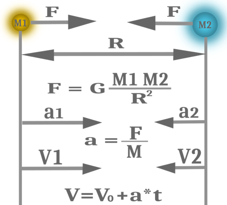
Figure 1. Force of gravity, acceleration and speed

The position of the particles provides the solution to the problem, while the fitness function is used to calculate the masses. The algorithm has two stages: exploration and exploitation. This algorithm uses intelligence capabilities at the beginning to avoid getting stuck in the local optimum, and after that it exploits the regions of extrema.

The gravitational search algorithm must turn a particle moving in space into an object with a certain mass. These objects are attracted due to the gravitational interaction with each other, and every particle in space will be attracted due to the mutual attraction of particles creating accelerations. Each particle is attracted by other particles and moves in the direction of the force. Particles with a small mass move towards particles with a larger mass, but massive objects also move, but at a lower speed inversely proportional to the mass. The optimal solution is found by "large" objects, which refine the solution by moving at a low speed compared to "smaller" objects that move more quickly. GSA implements the transfer of information through the interaction between objects.

GSA steps:

1. Agent initialization
2. Fitness evolution
3. Calculation of the gravitational constant
4. Calculation of agent masses

1. Agent initialization.
All agents are initialized randomly. Each agent is considered as a candidate solution. In order for the stability analysis to be meaningful and reliable, it is extremely important to specify the equilibrium initial conditions. After all, if the original "disk" of objects is not in equilibrium, its relaxation at the first time steps of the simulation can cause instabilities that are of little importance for our understanding of the stability of "disk galaxies". Unfortunately, no analytical solution is known for the density, velocity field and temperature of a three-dimensional gaseous disk in hydrostatic equilibrium in the external potential of the dark matter halo and/or stellar disk.

2. Fitness evolution.
The reliability and effectiveness of the GSA depends on the balance between research and exploitation capabilities. In the initial iterations of the solution search process, preference is given to exploring the search space. This can be achieved by allowing agents to use large step sizes in early iterations. In later iterations, refinement of the search space is required to avoid the situation of missing global optima. Thus, candidate solutions should have small step sizes to be used in subsequent iterations.

3. Calculation of the gravitational constant.
The gravitational constant (also known as the universal gravitational constant, the Newtonian constant of gravitation, or the Cavendish gravitational constant), denoted by the letter G, is an empirical physical constant involved in the calculation of gravitational effects in Isaac Newton's law of universal gravitation and in Albert Einstein's theory of general relativity. In Newton's law, it is the proportionality constant connecting the gravitational force between two bodies with the product of their masses and the inverse square of their distance. In the Einstein field equations, it quantifies the relation between the geometry of spacetime and the energy–momentum tensor.

4. Calculation of agent masses.
Mass is the amount of matter present in space.

Algorithm pseudocode:

1. generating a system of objects randomly.
2. determining the fitness of each object.
3. updating the values of the gravitational constant, calculating the masses, the best and the worst object.
4. calculation of forces acting on each coordinate.
5. calculation of accelerations and velocities of objects.
6. updating the positions of objects.
7. determining the fitness of each object.
8. repeat from p.3 until the termination criterion is met.

Let's consider the GSA code. To describe an object in the system of gravitational interaction, we need the S_Object structure, which will describe all the necessary physical properties of the object sufficient to carry out a gravitational search: c [] - coordinates in the search space, v [] - velocity vector for each of the coordinates (the array dimension is the number of coordinates), M is the object mass (in GSA, mass is a relative value, which is a calculated value depending on the value of the maximum and minimum fitness over the entire system of objects), f is the value of fitness, R[] is the Euclidean distance to other objects (the dimension of the array is the number of objects), F [] is the vector of forces for each of the coordinates (the dimension of the array is the number of coordinates).

//——————————————————————————————————————————————————————————————————————————————
struct S_Object
{
  double c  [];   //coordinates
  double v  [];   //velocity
  double M;       //mass
  double f;       //fitness
  double R  [];   //euclidean distance to other objects
  double F  [];   //force vector
};
//——————————————————————————————————————————————————————————————————————————————

Let's declare the class of the gravitational search algorithm C_AO_GSA. Out of the physical properties of the objects participating in the algorithm as agents, only one thing is needed: the coordinates that represent the best solution - the value of fB. The class declares valid ranges of search space coordinates and a step. The system of gravitationally bound objects is represented as an array of S_Object structures. In the classical algorithm, there are only three external parameters: G_constant, a_constant, e_constant, which determine the properties of the gravitational interaction of objects, and the rest of the constants are included in the calculation equations, but I considered it appropriate to move these constants into the external parameters of the algorithm, which allows more flexible adjustment of the properties of the algorithm as a whole. I will consider all the parameters in more detail a bit later since they greatly affect the behavior of the algorithm.

//——————————————————————————————————————————————————————————————————————————————
class C_AO_GSA
{
  //----------------------------------------------------------------------------
  public: S_Object o       []; //object
  public: double rangeMax  []; //maximum search range
  public: double rangeMin  []; //manimum search range
  public: double rangeStep []; //step search
  public: double cB        []; //best coordinates
  public: double fB;           //FF of the best coordinates

  public: void Init (const int    coordinatesNumberP, //coordinates number
                     const int    objectsNumberP,     //objects number
                     const double PowerOfdistanceP,   //power of distance
                     const double GraviPert_MinP,     //gravitational perturbation Min
                     const double GraviPert_MaxP,     //gravitational perturbation Min
                     const double VelocityPert_MinP,  //Velocity perturbation Min
                     const double VelocityPert_MaxP,  //Velocity perturbation Max
                     const double G_constantP,        //G constant
                     const double a_constantP,        //a constant
                     const double e_constantP,        //e constant
                     const int    maxIterationsP);    //max Iterations

  public: void Moving   (int iter);
  public: void Revision ();

  //----------------------------------------------------------------------------
  private: int    coordinatesNumber; //coordinates number
  private: int    objectsNumber;     //objects number
  private: double PowerOfdistance;   //power of distance
  private: double GraviPert_Min;     //gravitational perturbation Min
  private: double GraviPert_Max;     //gravitational perturbation Min
  private: double VelocPert_Min;     //velocity perturbation Min
  private: double VelocPert_Max;     //velocity perturbation Max
  private: double G_constant;        //G constant
  private: double a_constant;        //a constant
  private: double e_constant;        //e constant
  private: int    maxIterations;
  private: bool   revision;

  private: double SeInDiSp  (double In, double InMin, double InMax, double Step);
  private: double RNDfromCI (double min, double max);
  private: double Scale     (double In, double InMIN, double InMAX, double OutMIN, double OutMAX,  bool revers);
};
//——————————————————————————————————————————————————————————————————————————————

The public method of the Init () algorithm is intended for passing the external parameters of the algorithm to internal constants for initializing service variables and assigning sizes to arrays.

//——————————————————————————————————————————————————————————————————————————————
void C_AO_GSA::Init (const int    coordinatesNumberP, //coordinates number
                     const int    objectsNumberP,     //objects number
                     const double PowerOfdistanceP,   //power of distance
                     const double GraviPert_MinP,     //gravitational perturbation Min
                     const double GraviPert_MaxP,     //gravitational perturbation Min
                     const double VelocityPert_MinP,  //Velocity perturbation Min
                     const double VelocityPert_MaxP,  //Velocity perturbation Max
                     const double G_constantP,        //G constant
                     const double a_constantP,        //a constant
                     const double e_constantP,        //e constant
                     const int    maxIterationsP)     //max Iterations
{
  MathSrand ((int)GetMicrosecondCount ()); // reset of the generator
  fB       = -DBL_MAX;
  revision = false;

  coordinatesNumber = coordinatesNumberP;
  objectsNumber     = objectsNumberP;
  PowerOfdistance   = PowerOfdistanceP;
  GraviPert_Min     = GraviPert_MinP;
  GraviPert_Max     = GraviPert_MaxP;
  VelocPert_Min     = VelocityPert_MinP;
  VelocPert_Max     = VelocityPert_MaxP;
  G_constant        = G_constantP;
  a_constant        = a_constantP;
  e_constant        = e_constantP;
  maxIterations     = maxIterationsP;

  ArrayResize (rangeMax,  coordinatesNumber);
  ArrayResize (rangeMin,  coordinatesNumber);
  ArrayResize (rangeStep, coordinatesNumber);

  ArrayResize (o,  objectsNumber);

  for (int i = 0; i < objectsNumber; i++)
  {
    ArrayResize (o [i].c,  coordinatesNumber);
    ArrayResize (o [i].v,  coordinatesNumber);
    ArrayResize (o [i].R,  objectsNumber);
    ArrayResize (o [i].F,  coordinatesNumber);
    o [i].f  = -DBL_MAX;
  }

  ArrayResize (cB, coordinatesNumber);
}
//——————————————————————————————————————————————————————————————————————————————

The first public method called on each iteration of the Moving () iteration. This method contains all the physics and logic of the GSA algorithm. It is quite large, so let's consider it, breaking it into parts. Note that the method takes the current iteration as a parameter, the parameter is involved in the calculation of the gravitational constant, adjusting the balance between research and exploitation.

At the first iteration, the object initialization stage occurs. For all coordinates of objects, we assign random values in the allowable range with a uniform distribution, as well as check for out of range. At the beginning of the optimization process, all objects have zero velocity, that is, the objects are motionless in the search space with respect to coordinates. Note that objects have no mass, so they would have to move at the speed of light, but we will break the laws of physics for the first iteration, because this moment is to some extent equivalent to the Big Bang. The fitness of objects at this moment is the smallest of the possible values of the 'double' number. When debugging the algorithm, it was difficult to find bugs related to zero mass, you can see the solution below.

//----------------------------------------------------------------------------
if (!revision)
{
  fB = -DBL_MAX;

  for (int obj = 0; obj < objectsNumber; obj++)
  {
    for (int c = 0; c < coordinatesNumber; c++)
    {
      o [obj].c [c] = RNDfromCI (rangeMin [c], rangeMax [c]);
      o [obj].c [c] = SeInDiSp (o [obj].c [c], rangeMin [c], rangeMax [c], rangeStep [c]);
      o [obj].v [c] = 0.0;
      o [obj].M     = 0.0;
      o [obj].f     = -DBL_MAX;
    }
  }

  revision = true;
}

The rest of the code for the Moving () method refers to the second and subsequent iterations, where objects will gain mass, speed and acceleration.

First of all, we need to calculate the mass. As mentioned above, the mass (a positive scalar value by definition) of objects is calculated from the values of the fitness function, so it is necessary to determine the minimum and maximum fitness values prior to calculating the mass based on the obtained values. By this moment, the value of the fitness function has already been obtained at the previous iteration.

//find the minimum and maximum fitness==========================================
for (int obj = 0; obj < objectsNumber; obj++)
{
  if (o [obj].f < Fmin) Fmin = o [obj].f;
  if (o [obj].f > Fmax) Fmax = o [obj].f;
}

At this point in the code, the mass is calculated using the equation Mo=(Fo-Fmin)/(Fmax-Fmin), where:

• Mo - object mass
• Fo - object fitness
• Fmax - maximum fitness value among all objects (best value)
• Fmin - minimum fitness value among all objects (worst value)
  

As we can see from the equation, the mass can only take positive values in the range from 0 to 1 inclusive. Since we discussed earlier that the mass must not be equal to zero, otherwise the speed will be equal to the speed of light, we will limit the lower limit of the mass to 0.1. The upper value may well be equal to 1. Also, keep in mind that if the minimum and maximum values of the fitness function are equal, the mass of all objects will be the same for all and equal to 1. This corresponds to the case when the search space is homogeneous in the area where the objects are located and all objects are equal in terms of the quality of the fitness function, as well as movement in any direction has an equal priority. It would seem that in this case all objects should gradually move and concentrate towards a common center of mass, but this does not happen due to the non-linear action of the gravitational force.

//calculating the mass of objects===========================================
for (int obj = 0; obj < objectsNumber; obj++)
{
  Fo = o [obj].f;
  if (Fmax == Fmin) Mo = 1.0;
  else Mo = (Fo - Fmin) / (Fmax - Fmin);
  o [obj].M = Scale (Mo, 0.0, 1.0, 0.1, 1.0, false);
}

We have calculated the mass for the objects, now it is necessary to calculate one more component of the R equation - the Euclidean distance from each object to every other object. The calculation consists of two cycles of enumeration of objects and a cycle of calculation for each of the coordinates. As we remember, the Euclidean distance is the root of the sum of the squares of the coordinate differences.

//calculation of Euclidean distances between all objects====================
for (int obj = 0; obj < objectsNumber; obj++) ArrayInitialize (o [obj].R, 0.0);

for (int obj = 0; obj < objectsNumber; obj++)
{
  for (int obj2 = 0; obj2 < objectsNumber; obj2++)
  {
    if (obj != obj2)
    {
      if (o [obj].R [obj2] == 0.0)
      {
        for (int c = 0; c < coordinatesNumber; c++)
        {
          diffDist = o [obj].c [c] - o [obj2].c [c];
          o [obj].R [obj2] += diffDist * diffDist;
        }

        o [obj].R [obj2] = sqrt (o [obj].R [obj2]);
        o [obj2].R [obj] = o [obj].R [obj2];
      }
    }
  }
}

Now we can calculate force vectors for objects. To do this, we also need to go through all the objects in two cycles and one cycle for the coordinates, since the speed is calculated separately for each coordinate. We must add a condition that excludes the coincidence of object indexes so that the object excludes the calculation of itself in the force calculation. Here we use Newton's well-known equation to calculate the gravitational force for two objects (Figure 1) correcting the distance by the e_constant ratio. Let us first calculate the gravitational constant G, which should change downwards at each iteration assuming that the algorithm intensifies by the end of the optimization.

//calculate the force vector for each object================================
for (int obj = 0; obj < objectsNumber; obj++) ArrayInitialize (o [obj].F, 0.0);

double G = G_constant * exp (-a_constant * (iter / maxIterations));

for (int obj = 0; obj < objectsNumber; obj++)
{
  for (int obj2 = 0; obj2 < objectsNumber; obj2++)
  {
    if (obj != obj2)
    {
      for (int c = 0; c < coordinatesNumber; c++)
      {
        diffDist = o [obj2].c [c] - o [obj].c [c];

        if (o [obj].R [obj2] != 0.0)
        {
          o [obj] .F [c] += G * o [obj].M * o [obj2].M * diffDist / (pow (o [obj].R [obj2], PowerOfdistance) + e_constant);
        }
      }
    }
  }
}

Now we only need to calculate the speed in order for the objects to start moving. From the equation in Figure 1, we can see that speed calculation involves acceleration, while acceleration is equal to the force acting on the body divided by the mass. The equation also contains the time V=V0+a*t. In our algorithm, iteration plays the role of time, so the change in speed is nothing more than an increase in speed in one iteration. The velocity vector has already been calculated above. It remains to divide by the mass. In addition, the authors introduce force perturbation and velocity perturbation. The perturbation is a uniformly distributed random number between 0 and 1. This adds a random component to the movement of objects, without which the movement would be strictly determined and would depend only on the initial position of the bodies. I considered it reasonable to bring the perturbation indicators into the external parameters of the algorithm, which will allow to regulate the movement of objects from completely deterministic to completely random.

//calculation of acceleration and velocity for all objects==================
double a = 0.0; //acceleration

for (int obj = 0; obj < objectsNumber; obj++)
{
  for (int c = 0; c < coordinatesNumber; c++)
  {
    r = RNDfromCI (GraviPert_Min, GraviPert_Max);
    a = o [obj].F [c] * r / o [obj].M;
    r = RNDfromCI (GraviPert_Min, GraviPert_Max);
    o [obj].v [c] = o [obj].v [c] * r + a;
    o [obj].c [c] = o [obj].c [c] + o [obj].v [c];

    if (o [obj].c [c] > rangeMax [c]) o [obj].c [c] = rangeMin [c];
    if (o [obj].c [c] < rangeMin [c]) o [obj].c [c] = rangeMax [c];

    o [obj].c [c] = SeInDiSp (o [obj].c [c], rangeMin [c], rangeMax [c], rangeStep [c]);
  }
}

The second Revision () method, which is mandatory for execution at each iteration. The method is designed to determine the best fitness value for the current iteration. In the loop, go through all the objects and replace the global best solution.

//——————————————————————————————————————————————————————————————————————————————
void C_AO_GSA::Revision ()
{
  for (int s = 0; s < objectsNumber; s++)
  {
    if (o [s].f > fB)
    {
      fB = o [s].f;
      ArrayCopy (cB, o [s].c, 0, 0, WHOLE_ARRAY);
    }
  }
}
//——————————————————————————————————————————————————————————————————————————————

3. Test results

Let's move on to the test results. Below are the test stand results with the best GSA parameters I could find:

2023.02.03 14:12:43.440    Test_AO_GSA (EURUSD,M1)    C_AO_GSA:10;2.0;0.2;0.6;0.0;1.0;2.0;20.0;0.01
2023.02.03 14:12:43.440    Test_AO_GSA (EURUSD,M1)    =============================
2023.02.03 14:12:52.198    Test_AO_GSA (EURUSD,M1)    5 Rastrigin's; Func runs 10000 result: 73.64619475145881
2023.02.03 14:12:52.198    Test_AO_GSA (EURUSD,M1)    Score: 0.91252
2023.02.03 14:13:06.105    Test_AO_GSA (EURUSD,M1)    25 Rastrigin's; Func runs 10000 result: 59.4327218024363
2023.02.03 14:13:06.105    Test_AO_GSA (EURUSD,M1)    Score: 0.73640
2023.02.03 14:14:16.529    Test_AO_GSA (EURUSD,M1)    500 Rastrigin's; Func runs 10000 result: 37.550565227034724
2023.02.03 14:14:16.529    Test_AO_GSA (EURUSD,M1)    Score: 0.46527
2023.02.03 14:14:16.529    Test_AO_GSA (EURUSD,M1)    =============================
2023.02.03 14:14:30.577    Test_AO_GSA (EURUSD,M1)    5 Forest's; Func runs 10000 result: 0.741456333008312
2023.02.03 14:14:30.577    Test_AO_GSA (EURUSD,M1)    Score: 0.41941
2023.02.03 14:14:50.281    Test_AO_GSA (EURUSD,M1)    25 Forest's; Func runs 10000 result: 0.46894018717768426
2023.02.03 14:14:50.282    Test_AO_GSA (EURUSD,M1)    Score: 0.26526
2023.02.03 14:16:01.856    Test_AO_GSA (EURUSD,M1)    500 Forest's; Func runs 10000 result: 0.11382493516764165
2023.02.03 14:16:01.856    Test_AO_GSA (EURUSD,M1)    Score: 0.06439
2023.02.03 14:16:01.856    Test_AO_GSA (EURUSD,M1)    =============================
2023.02.03 14:16:18.195    Test_AO_GSA (EURUSD,M1)    5 Megacity's; Func runs 10000 result: 5.279999999999999
2023.02.03 14:16:18.195    Test_AO_GSA (EURUSD,M1)    Score: 0.44000
2023.02.03 14:16:34.536    Test_AO_GSA (EURUSD,M1)    25 Megacity's; Func runs 10000 result: 2.296
2023.02.03 14:16:34.536    Test_AO_GSA (EURUSD,M1)    Score: 0.19133
2023.02.03 14:17:46.887    Test_AO_GSA (EURUSD,M1)    500 Megacity's; Func runs 10000 result: 0.23399999999999999
2023.02.03 14:17:46.887    Test_AO_GSA (EURUSD,M1)    Score: 0.01950

Algorithm parameters:

input double PowerOfdistance_P  = 2.0;   //Power of distance
input double GraviPert_Min_P    = 0.2;   //Gravitational perturbation Min
input double GraviPert_Max_P    = 0.6;   //Gravitational perturbation Max
input double VelocityPert_Min_P = 0.0;   //Velocity perturbation Min
input double VelocityPert_Max_P = 1.0;   //Velocity perturbation Max
input double G_constant_P       = 2.0;   //G constant
input double a_constant_P       = 20.0;  //a constant
input double e_constant_P       = 0.01;  //e constant

PowerOfdistance_P - degree, to which we raise the distance between objects, affects the formation of gravitationally bound objects. the higher the degree in the equation, the less impact objects have on other objects.

• GraviPert_Min_P - lower limit of the gravitational perturbation range.
• GraviPert_Max_P - upper limit of the gravitational perturbation range.
• In case of GraviPert_Min_P = 1.0 and GraviPert_Max_P = 1.0, there is no gravitational disturbance.
• VelocityPert_Min_P - lower limit of the velocity perturbation range.
• VelocityPert_Max_P - upper limit of the velocity perturbation range.

In case of VelocityPert_Min_P = 1.0 and VelocityPert_Max_P = 1.0, there is no velocity perturbation.

• G_constant_P - gravitational constant acts as a scale factor: the higher the value, the stronger the gravitational forces act and the faster the speed of objects changes.
• a_constant_P - correction factor for the gravitational constant designed to reduce the search field during the entire optimization in order to refine the found extrema.
• e_constant_P - correction factor for distance between objects.

Let's take a look at the visualization test results. The behavior of the algorithm on test functions is very peculiar and interesting. In fact, the experiment displays the work of gravitational forces. The movement of objects and the obtained optimization results are strongly influenced by the external parameters of the algorithm. Initially, objects with zero speed are randomly distributed over the search space and start moving at the next iteration. The settings, which were used in testing (the best I found), make objects move towards a common center of mass.

Do not forget that the gravity of each object affects other objects, the laws of motion of which are described with sufficiently high accuracy in the algorithm. Approaching the common center of mass, the objects continue to move at a high speed. It looks like a pulsating movement of a mass of particles towards the common center of mass and back. After a certain number of iterations, the movement of objects changes its trajectory under the influence of the space relief of the fitness function, which acts as a gravitational inhomogeneity affecting the mass of objects. As we discussed earlier, the mass of objects is calculated from the value of the fitness function. However, the Rastrigin function, which is symmetrical along the axes, has a fairly uniform effect on the movement of objects, and the breakdown into groups is not particularly noticeable.

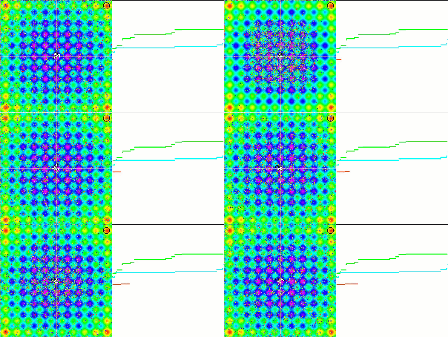
  GSA on the Rastrigin test function.

Even more interesting behavior is shown by the objects in the Forest and Megacity functions. These functions are not symmetrical and therefore have a non-uniform effect on the entire group of objects.

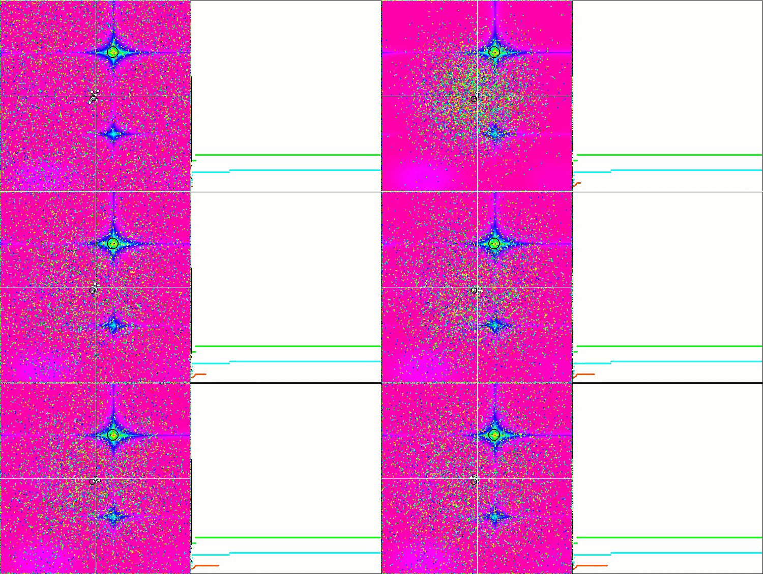
  GSA on the Forest test function.

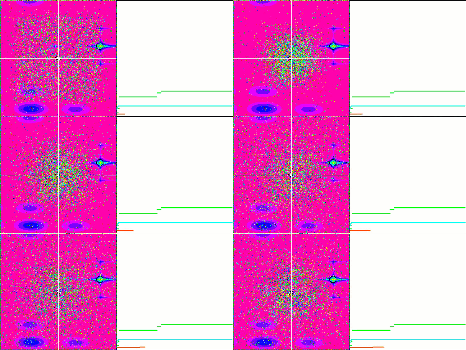
GSA on the Megacity test function.

After a lot of experimentation with GSA, I came up with the idea to make a simulator of space objects movement. It has no practical value, but it gives an idea of the physical laws acting on planetary and stellar systems. The simulator is a version of the GSA with randomness disabled. Additionally, three objects imitating three stars (a blue giant, a yellow star and a white dwarf), are introduced. The mass parameters are displayed separately in the settings for them.

A new Universe fitness function has been created with a uniform space specially for the simulator. The simulator clearly shows how the degree (parameter) of the distance between objects affects their mutual movement. In the visualization below, a power of 3 is applied instead of the standard value of Newton's law of 2. It becomes clear how the degree affects the formation of gravitationally bound systems, such as pair and triple star systems.

If in our universe the degree of distance had been higher, then galaxies would have formed much earlier than in reality. The animation clearly shows that paired objects circulating around a common center of mass appeared at the very first iterations. As expected, the blue giant collected the most objects around it.

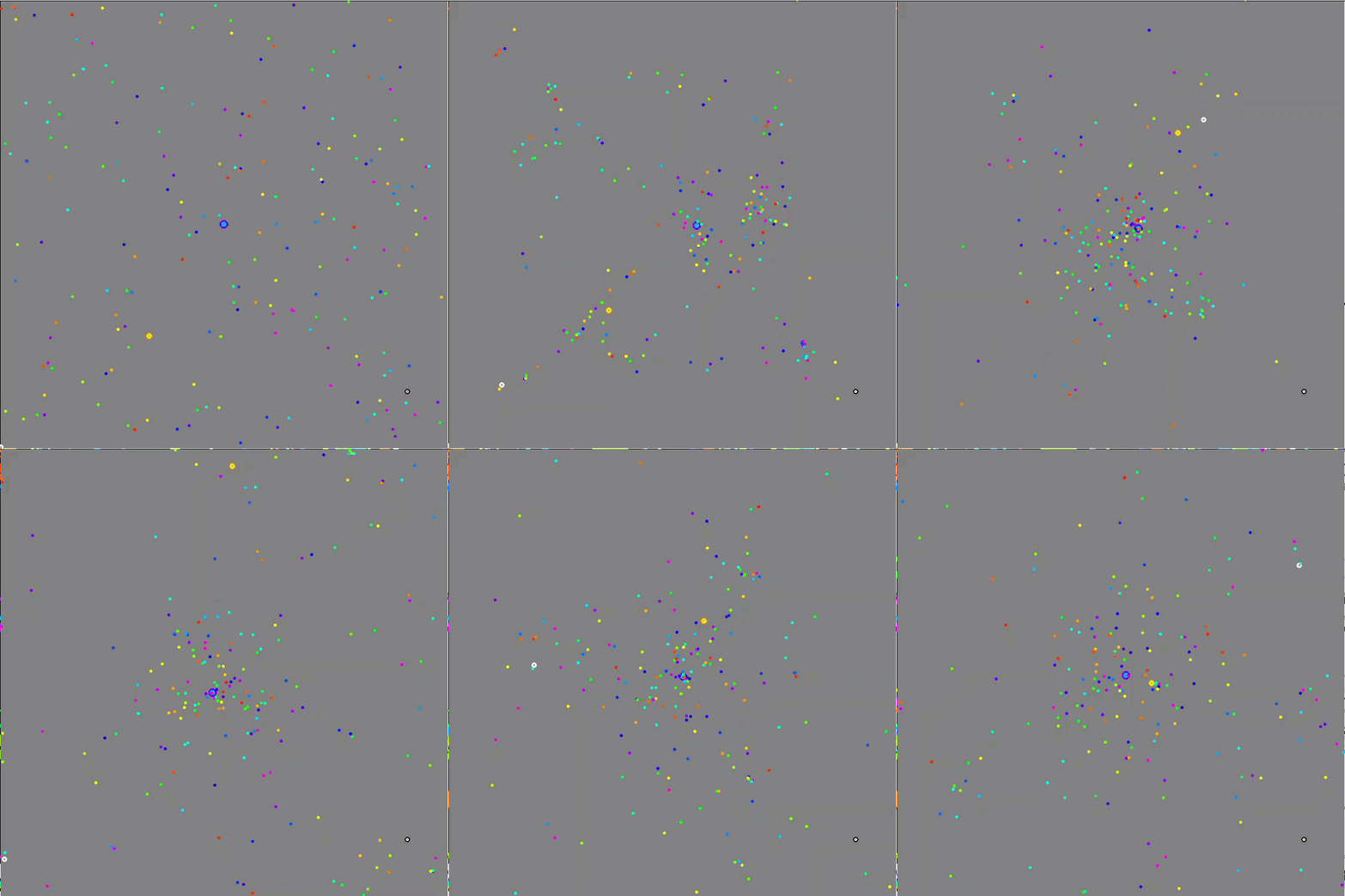
Visualization of the space objects movement simulator based on the GSA algorithm

Let's move on to the analysis of the GSA test results. The original features used in the algorithm did not allow it to achieve strong results in our testing. Numerous variations of the parameters that I tried did not improve the convergence of the algorithm. The algorithm showed some positive results relative to other test participants on the smooth Rastrigin function with 10 variables and Megacity. In other tests, GSA performs below the average in the table taking 8th place out of 12.

AO	Description	Rastrigin			Rastrigin final	Forest			Forest final	Megacity (discrete)			Megacity final	Final result
		10 params (5 F)	50 params (25 F)	1000 params (500 F)		10 params (5 F)	50 params (25 F)	1000 params (500 F)		10 params (5 F)	50 params (25 F)	1000 params (500 F)
IWO	invasive weed optimization	1.00000	1.00000	0.35295	2.35295	0.79937	0.46349	0.41071	1.67357	0.75912	0.44903	0.94416	2.15231	100.000
ACOm	ant colony optimization M	0.36118	0.26810	0.20182	0.83110	1.00000	1.00000	1.00000	3.00000	1.00000	1.00000	0.15901	2.15901	96.805
COAm	cuckoo optimization algorithm M	0.96423	0.69756	0.30792	1.96971	0.64504	0.34034	0.21362	1.19900	0.67153	0.34273	0.48451	1.49877	74.417
FAm	firefly algorithm M	0.62430	0.50653	0.20290	1.33373	0.55408	0.42299	0.64360	1.62067	0.21167	0.28416	1.00000	1.49583	70.740
BA	bat algorithm	0.42290	0.95047	1.00000	2.37337	0.17768	0.17477	0.33595	0.68840	0.15329	0.07158	0.49268	0.71755	59.383
ABC	artificial bee colony	0.81573	0.48767	0.24656	1.54996	0.58850	0.21455	0.17249	0.97554	0.47444	0.26681	0.39496	1.13621	57.393
BFO	bacterial foraging optimization	0.70129	0.46155	0.13988	1.30272	0.41251	0.26623	0.26695	0.94569	0.42336	0.34491	0.53694	1.30521	55.563
GSA	gravitational search algorithm	0.73222	0.67404	0.00000	1.40626	0.31238	0.36416	0.42921	1.10575	0.51095	0.36658	0.00000	0.87753	52.786
FSS	fish school search	0.48850	0.37769	0.13383	1.00002	0.78060	0.05013	0.08423	0.91496	0.00000	0.01084	0.23493	0.24577	20.094
PSO	particle swarm optimisation	0.21339	0.12224	0.08478	0.42041	0.15345	0.10486	0.28099	0.53930	0.08028	0.02385	0.05550	0.15963	14.358
RND	random	0.17559	0.14524	0.09495	0.41578	0.08623	0.04810	0.06094	0.19527	0.00000	0.00000	0.13960	0.13960	8.117
GWO	grey wolf optimizer	0.00000	0.00000	0.02672	0.02672	0.00000	0.00000	0.00000	0.00000	0.18977	0.04119	0.07252	0.30348	1.000

In general, the GSA algorithm is noticeably sensitive to the presence of a gradient in the function being optimized. Low scalability does not allow it to be used for serious tasks containing many variables, so I would not recommend the algorithm for use with neural networks and for optimizing trading systems. I have not fully studied the possibilities of the gravitational search algorithm. Additional research may open new unknown positive features of this very interesting and unusual algorithm. The main advantages of the algorithm are independence from the current best found global solution and the ability of all agents to interact with each other. 

Fig. 2 shows the test results of the algorithm

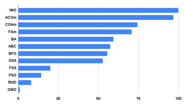
Figure 2. Histogram of the test results of the algorithms

Conclusions on the properties of the Gravitational Search Algorithm (GSA):

Pros:
1. Easy implementation.
2. Good performance on smooth functions with few variables.

Cons:
1. High computational complexity.
2. Poor results on discrete functions.
3. Bad scalability.