Using PSAR, Heiken Ashi, and Deep Learning Together for Trading

Introduction

Finding an edge can be the difference between success and failure. With so much data available, traders are increasingly turning to advanced technologies like deep learning to gain an advantage. This journey involves combining traditional technical analysis tools with modern artificial intelligence (AI) models to quickly assess and adapt to market conditions. To explore this potential, we've developed a Python script designed to blend the predictive power of deep learning with tried-and-true trading indicators. This script isn't intended to be a full-blown trading system; rather, it's a tool for rapid experimentation—a way to quickly test if a trading strategy has the potential to be profitable. In parallel, a MetaTrader 5 script uses similar principles to bring this approach into a live trading environment, bridging the gap between theoretical backtesting and real-world application.

Making the Deep Learning ONNX model

In the fast-paced world of forex trading, staying ahead of the curve is crucial. That's why we've developed a Python script that harnesses the power of deep learning to predict currency pair movements. Let's take a friendly tour through this exciting piece of code and see how it works its magic!

Our script begins by importing all the necessary tools - think of it as gathering ingredients for a complex recipe. We're using libraries like TensorFlow and Keras, which are the powerhouses behind many modern AI applications. We're also using MetaTrader 5 to fetch real forex data.

import MetaTrader5 as mt5
import tensorflow as tf
import numpy as np
import pandas as pd
import tf2onnx
import keras

Next, we set up some important parameters. We're looking at 120 days of historical data for the EURUSD pair. Why 120? It's a sweet spot that gives us enough history to spot patterns without overwhelming our model.

We then use MetaTrader 5 to fetch this data. Imagine it as sending a time traveler back to collect price information from the past 120 days. Once we have this data, we organize it neatly into a format our AI can understand.

inp_history_size = 120

sample_size = inp_history_size*3*20
symbol = "EURUSD"
optional = "D1_2024"
inp_model_name = str(symbol)+"_"+str(optional)+".onnx" 

if not mt5.initialize():
    print("initialize() failed, error code =",mt5.last_error())
    quit()

# we will save generated onnx-file near the our script to use as resource
from sys import argv
data_path=argv[0]
last_index=data_path.rfind("\\")+1
data_path=data_path[0:last_index]
print("data path to save onnx model",data_path)

# and save to MQL5\Files folder to use as file
terminal_info=mt5.terminal_info()
file_path=terminal_info.data_path+"\\MQL5\\Files\\"
print("file path to save onnx model",file_path)

# set start and end dates for history data
from datetime import timedelta, datetime
#end_date = datetime.now()
end_date = datetime(2024, 1, 1, 0)
start_date = end_date - timedelta(days=inp_history_size*20*3)

# print start and end dates
print("data start date =",start_date)
print("data end date =",end_date)

# get rates
eurusd_rates = mt5.copy_rates_from(symbol, mt5.TIMEFRAME_D1, end_date, sample_size)

Raw financial data can be messy, so we clean it up. We focus on the closing prices - that's the final price of each trading day. We also scale this data to be between 0 and 1. This step is crucial because it helps our AI model learn more effectively, kind of like translating everything into a common language.

from sklearn.preprocessing import MinMaxScaler
scaler=MinMaxScaler(feature_range=(0,1))
scaled_data = scaler.fit_transform(data)

We don't want our model to memorize the data, so we split it into two parts: training data (80%) and testing data (20%). It's like giving our AI student a textbook to study from (training data) and then a separate quiz to test its knowledge (testing data).

# scale data
from sklearn.preprocessing import MinMaxScaler
scaler=MinMaxScaler(feature_range=(0,1))
scaled_data = scaler.fit_transform(data)

# training size is 80% of the data
training_size = int(len(scaled_data)*0.80) 
print("Training_size:",training_size)
train_data_initial = scaled_data[0:training_size,:]
test_data_initial = scaled_data[training_size:,:1]

# split a univariate sequence into samples
def split_sequence(sequence, n_steps):
    X, y = list(), list()
    for i in range(len(sequence)):
       # find the end of this pattern
       end_ix = i + n_steps
       # check if we are beyond the sequence
       if end_ix > len(sequence)-1:
          break
       # gather input and output parts of the pattern
       seq_x, seq_y = sequence[i:end_ix], sequence[end_ix]
       X.append(seq_x)
       y.append(seq_y)
    return np.array(X), np.array(y)

# split into samples
time_step = inp_history_size
x_train, y_train = split_sequence(train_data_initial, time_step)
x_test, y_test = split_sequence(test_data_initial, time_step)

# reshape input to be [samples, time steps, features] which is required for LSTM
x_train =x_train.reshape(x_train.shape[0],x_train.shape[1],1)
x_test = x_test.reshape(x_test.shape[0],x_test.shape[1],1)

Now comes the exciting part - building our AI model! We're using a combination of different AI techniques:

1.  Convolutional Neural Networks (CNNs): These are great at spotting patterns in sequences, just like how our eyes spot patterns in images.
2.  Long Short-Term Memory (LSTM) networks: These are excellent at understanding long-term dependencies in data, perfect for spotting trends over time.
3.  Dense layers: These help our model make its final predictions.

We also add some dropout layers to prevent our model from becoming overconfident and "overfitting" the data.

# define model
from keras.models import Sequential
from keras.layers import Dense, Activation, Conv1D, MaxPooling1D, Dropout, Flatten, LSTM
from keras.metrics import RootMeanSquaredError as rmse
from tensorflow.keras import callbacks
model = Sequential()
model.add(Conv1D(filters=256, kernel_size=2, strides=1, padding='same', activation='relu', input_shape=(inp_history_size,1)))
model.add(MaxPooling1D(pool_size=2))
model.add(LSTM(100, return_sequences = True))
model.add(Dropout(0.3))
model.add(LSTM(100, return_sequences = False))
model.add(Dropout(0.3))
model.add(Dense(units=1, activation = 'sigmoid'))
model.compile(optimizer='adam', loss= 'mse' , metrics = [rmse()])

# Set up early stopping
early_stopping = callbacks.EarlyStopping(
    monitor='val_loss',
    patience=20,
    restore_best_weights=True,
)

# model training for 300 epochs
history = model.fit(x_train, y_train, epochs = 300 , validation_data = (x_test,y_test), batch_size=32, callbacks=[early_stopping], verbose=2)

Training the model is like sending our AI to school. We show it our training data many times (up to 300 epochs), and it gradually learns to predict future prices based on past patterns. We use something called "early stopping" to make sure our AI doesn't study for too long and start memorizing instead of learning.

After training, we test our model's performance. We use metrics like RMSE (Root Mean Square Error) to see how close our predictions are to the actual prices. It's like grading our AI's test results.

# evaluate training data
train_loss, train_rmse = model.evaluate(x_train,y_train, batch_size = 32)
print(f"train_loss={train_loss:.3f}")
print(f"train_rmse={train_rmse:.3f}")

# evaluate testing data
test_loss, test_rmse = model.evaluate(x_test,y_test, batch_size = 32)
print(f"test_loss={test_loss:.3f}")
print(f"test_rmse={test_rmse:.3f}")

The final step is converting our trained model to the ONNX format. ONNX is like a universal language for AI models - it allows our model to be used in different environments, including our MetaTrader scripts.

# Define a function that represents your model
@tf.function(input_signature=[tf.TensorSpec([None, inp_history_size, 1], tf.float32)])
def model_function(x):
    return model(x)

output_path = data_path+inp_model_name
# Convert the model to ONNX
onnx_model, _ = tf2onnx.convert.from_function(
    model_function, 
    input_signature=[tf.TensorSpec([None, inp_history_size, 1], tf.float32)],
    opset=13,
    output_path=output_path
)

print(f"Saved ONNX model to {output_path}")


# save model to ONNX
output_path = data_path+inp_model_name
onnx_model = tf2onnx.convert.from_keras(model, output_path=output_path)
print(f"saved model to {output_path}")

output_path = file_path+inp_model_name
onnx_model = tf2onnx.convert.from_keras(model, output_path=output_path)
print(f"saved model to {output_path}")

We don't just stop at numbers - we create several graphs to visualize how well our model is performing. These graphs show things like the model's learning progress and how its predictions compare to actual prices.

By the end of this script, we have a powerful ONNX model ready to be used in our forex trading strategies. It's trained on historical EURUSD data and can help predict future price movements.

Remember, while this model is sophisticated, it's not a crystal ball. The forex market is influenced by many complex factors. Always use AI predictions as one tool among many in your trading toolkit, and never forget the importance of risk management.

Python script to test a strategy

This Python script is essentially a quick way to test whether a trading strategy has the potential to be profitable. It’s not meant to be a fully-fledged trading system but rather a tool for rapid experimentation. By combining a deep learning model with technical analysis, it aims to see if there's a viable edge in the market without getting bogged down in complex optimizations right away.

The script starts by connecting to MetaTrader 5 to pull historical price data for EUR/USD. It uses hourly data to capture short-term movements and applies Heikin Ashi candlesticks to smooth out the noise in the market. This helps in identifying trends more clearly, which is crucial when you're quickly testing a strategy. It then layers on a few well-known technical indicators like PSAR, SMA, RSI, and ATR. These indicators serve as a quick check on market conditions, giving the model context for making buy and sell decisions.

import MetaTrader5 as mt5
import pandas as pd
import numpy as np
import onnxruntime as ort
from sklearn.preprocessing import MinMaxScaler
from ta.trend import PSARIndicator, SMAIndicator
from ta.momentum import RSIIndicator
from ta.volatility import AverageTrueRange
import matplotlib.pyplot as plt

# Inicializar conexión con MetaTrader5
if not mt5.initialize():
    print("Inicialización fallida")
    mt5.shutdown()

def get_historical_data(symbol, timeframe, start_date, end_date):
    rates = mt5.copy_rates_range(symbol, timeframe, start_date, end_date)
    df = pd.DataFrame(rates)
    df['time'] = pd.to_datetime(df['time'], unit='s')
    df.set_index('time', inplace=True)
    return df

def calculate_heikin_ashi(df):
    ha_close = (df['open'] + df['high'] + df['low'] + df['close']) / 4
    ha_open = (df['open'].shift(1) + df['close'].shift(1)) / 2
    ha_high = df[['high', 'open', 'close']].max(axis=1)
    ha_low = df[['low', 'open', 'close']].min(axis=1)
    
    df['ha_close'] = ha_close
    df['ha_open'] = ha_open
    df['ha_high'] = ha_high
    df['ha_low'] = ha_low
    return df

def add_indicators(df):
    # Calcular Heikin Ashi
    df = calculate_heikin_ashi(df)
    
    # PSAR con parámetros ajustados
    psar = PSARIndicator(df['high'], df['low'], df['close'], step=0.02, max_step=0.2)
    df['psar'] = psar.psar()
    
    # Añadir SMA
    sma = SMAIndicator(df['close'], window=50)
    df['sma'] = sma.sma_indicator()
    
    # Añadir RSI
    rsi = RSIIndicator(df['close'], window=14)
    df['rsi'] = rsi.rsi()
    
    # Añadir ATR para medir volatilidad
    atr = AverageTrueRange(df['high'], df['low'], df['close'], window=14)
    df['atr'] = atr.average_true_range()
    
    # Añadir filtro de tendencia simple
    df['trend'] = np.where(df['close'] > df['sma'], 1, -1)
    
    return df

The heart of the script lies in its use of a pre-trained ONNX deep learning model. By scaling the data and feeding it into this model, the script generates predictions on where the market might go next. It combines these predictions with the technical indicators to create a basic set of trading rules. For example, it looks for opportunities to go long when certain conditions align, like the price being above the moving average and the RSI showing that the market isn't overbought. Conversely, it signals a short position when the opposite conditions are met. The script even adds adaptive stop-loss and take-profit mechanisms to manage risk, although these are kept relatively simple to maintain the script's focus on rapid testing.

def prepare_data(df, window_size=120):
    scaler = MinMaxScaler(feature_range=(0, 1))
    scaled_data = scaler.fit_transform(df[['close']])
    
    X = []
    for i in range(window_size, len(scaled_data)):
        X.append(scaled_data[i-window_size:i])
    
    return np.array(X), scaler

def load_onnx_model(model_path):
    return ort.InferenceSession(model_path)

def predict_with_onnx(model, input_data):
    input_name = model.get_inputs()[0].name
    output_name = model.get_outputs()[0].name
    return model.run([output_name], {input_name: input_data})[0]

def backtest(df, model, scaler, window_size=120, initial_balance=10000):
    scaled_data = scaler.transform(df[['close']])
    
    predictions = []
    for i in range(window_size, len(scaled_data)):
        X = scaled_data[i-window_size:i].reshape(1, window_size, 1)
        pred = predict_with_onnx(model, X.astype(np.float32))
        predictions.append(scaler.inverse_transform(pred.reshape(-1, 1))[0, 0])
    
    df['predictions'] = [np.nan]*window_size + predictions
    
    # Nueva lógica de trading
    df['position'] = 0
    long_condition = (
        (df['close'] > df['predictions']) & 
        (df['close'] > df['psar']) & 
        (df['close'] > df['sma']) & 
        (df['rsi'] < 60) &  # Condición RSI menos estricta
        (df['ha_close'] > df['ha_open']) &
        (df['ha_close'].shift(1) > df['ha_open'].shift(1)) &
        (df['trend'] == 1)  # Solo comprar en tendencia alcista
    )
    short_condition = (
        (df['close'] < df['predictions']) & 
        (df['close'] < df['psar']) & 
        (df['close'] < df['sma']) & 
        (df['rsi'] > 40) &  # Condición RSI menos estricta
        (df['ha_close'] < df['ha_open']) &
        (df['ha_close'].shift(1) < df['ha_open'].shift(1)) &
        (df['trend'] == -1)  # Solo vender en tendencia bajista
    )
    
    df.loc[long_condition, 'position'] = 1  # Compra
    df.loc[short_condition, 'position'] = -1  # Venta
    
    # Implementar stop-loss y take-profit adaptativos
    sl_atr_multiple = 2
    tp_atr_multiple = 3
    
    for i in range(window_size, len(df)):
        if df['position'].iloc[i-1] != 0:
            entry_price = df['close'].iloc[i-1]
            current_atr = df['atr'].iloc[i-1]
            if df['position'].iloc[i-1] == 1:  # Posición larga
                sl_price = entry_price - sl_atr_multiple * current_atr
                tp_price = entry_price + tp_atr_multiple * current_atr
                if df['low'].iloc[i] < sl_price or df['high'].iloc[i] > tp_price:
                    df.loc[df.index[i], 'position'] = 0
            else:  # Posición corta
                sl_price = entry_price + sl_atr_multiple * current_atr
                tp_price = entry_price - tp_atr_multiple * current_atr
                if df['high'].iloc[i] > sl_price or df['low'].iloc[i] < tp_price:
                    df.loc[df.index[i], 'position'] = 0
    
    df['returns'] = df['close'].pct_change()
    df['strategy_returns'] = df['position'].shift(1) * df['returns']
    
    # Calcular balance
    df['cumulative_returns'] = (1 + df['strategy_returns']).cumprod()
    df['balance'] = initial_balance * df['cumulative_returns']
    
    return df

When it comes to results, the script gives a quick snapshot of the strategy's performance. In this case, it achieved a total return of 1.35%, meaning it turned $10,000 into $10,135.02 over the testing period. While this isn’t a spectacular gain, it's a positive outcome, suggesting that the strategy has some merit. The Sharpe Ratio, a common measure of risk-adjusted return, came in at 0.39. This figure indicates that while there were gains, they came with a fair amount of risk. For a quick test, this ratio is a useful way to gauge whether the strategy is worth pursuing further. 

Retorno total: 1.35%
Ratio de Sharpe: 0.39
Balance final: $10135.02

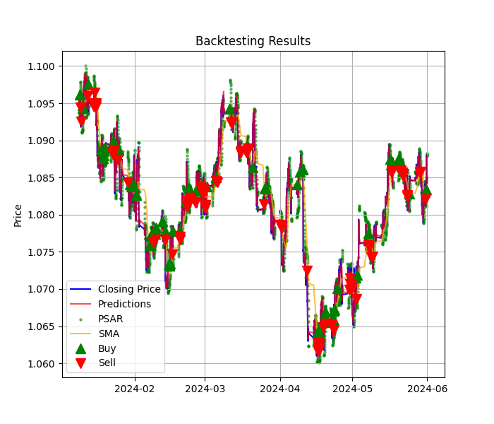
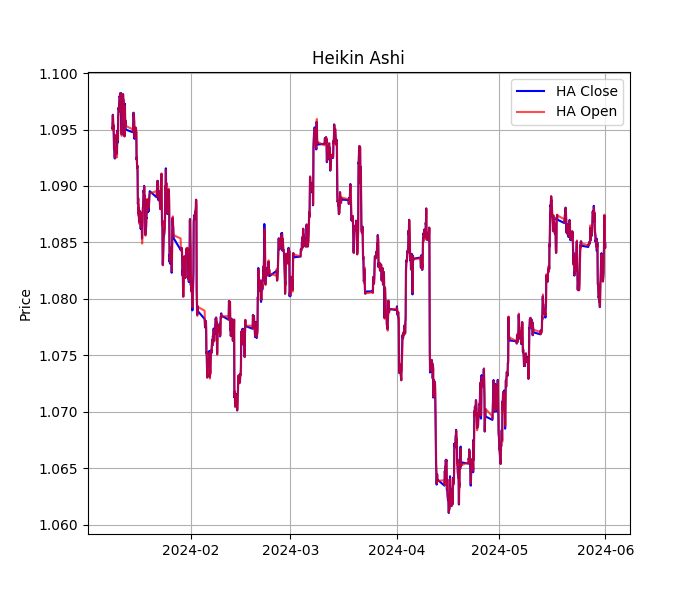
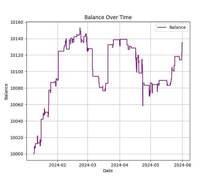
The visualizations generated by the script provide a helpful overview of how the strategy performed. The first graph shows the interplay between the market price, the model’s predictions, and the buy and sell signals. The Heikin Ashi chart offers a cleaner look at market trends, helping you see if the strategy is capturing the right moments to enter and exit trades. Lastly, the equity curve gives a straightforward look at how the account balance changed over time, highlighting both the periods of growth and the drawdowns.

In summary, this script is designed for quick experimentation. It helps you rapidly assess if a strategy has potential without diving too deep into fine-tuning. While it shows that the strategy can generate some profit, the modest Sharpe Ratio suggests there's still work to be done. This makes it a useful starting point—a way to quickly determine if a strategy is worth more in-depth development and optimization.

Expert Advisor

This MetaTrader 5 script is designed to quickly test whether a trading strategy can be profitable by using a mix of technical analysis and a deep learning model. The idea here is not to create a foolproof trading system but to experiment with combining traditional trading indicators with the power of machine learning to see if there's an edge in the market.

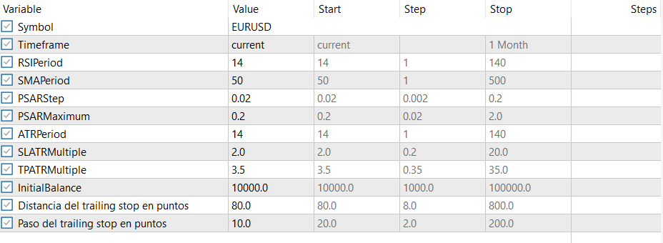
The script focuses on the EUR/USD currency pair and uses the H6 (6-hour) timeframe. It starts by setting up a handful of familiar technical indicators like the RSI, SMA, PSAR, and ATR. These are common tools traders use to gauge market momentum, trend direction, and volatility. On top of that, it uses Heikin Ashi candlesticks, which help smooth out price action and make trends easier to spot by reducing market noise. This initial setup lays the groundwork for what the script is trying to achieve: a systematic way to look for buy and sell opportunities.

int    handleRSI, handleSMA, handlePSAR, handleATR;
double rsiBuffer[], smaBuffer[], psarBuffer[], atrBuffer[];
double haOpen[], haClose[], haHigh[], haLow[];
CTrade trade;

   handleRSI = iRSI(Symbol, Timeframe, RSIPeriod, PRICE_CLOSE);
   handleSMA = iMA(Symbol, Timeframe, SMAPeriod, 0, MODE_SMA, PRICE_CLOSE);
   handlePSAR = iSAR(Symbol, Timeframe, PSARStep, PSARMaximum);
   handleATR = iATR(Symbol, Timeframe, ATRPeriod);

   if(handleRSI == INVALID_HANDLE || handleSMA == INVALID_HANDLE ||
      handlePSAR == INVALID_HANDLE || handleATR == INVALID_HANDLE)
     {
      Print("Error creating indicators");
      return(INIT_FAILED);
     }

   ArraySetAsSeries(rsiBuffer, true);
   ArraySetAsSeries(smaBuffer, true);
   ArraySetAsSeries(psarBuffer, true);
   ArraySetAsSeries(atrBuffer, true);

   ArrayResize(haOpen, 3);
   ArrayResize(haClose, 3);
   ArrayResize(haHigh, 3);
   ArrayResize(haLow, 3);
   ArraySetAsSeries(haOpen, true);
   ArraySetAsSeries(haClose, true);
   ArraySetAsSeries(haHigh, true);
   ArraySetAsSeries(haLow, true);

   IndicatorRelease(handleRSI);
   IndicatorRelease(handleSMA);
   IndicatorRelease(handlePSAR);
   IndicatorRelease(handleATR);

What sets this script apart is its use of a pre-trained ONNX deep learning model. Instead of relying solely on traditional technical analysis, the script taps into the predictive power of machine learning to forecast price movements. It loads this model directly into the trading environment, where it takes in recent market data, normalizes it, and predicts whether the price will move up, down, or stay the same. This prediction is then classified into one of three categories: an upward movement, a downward movement, or no significant movement at all. By blending these predictions with technical indicators, the script aims to make more informed trading decisions.

#define SAMPLE_SIZE 120

long     ExtHandle=INVALID_HANDLE;
int      ExtPredictedClass=-1;
datetime ExtNextBar=0;
datetime ExtNextDay=0;
float    ExtMin=0.0;
float    ExtMax=0.0;
CTrade   ExtTrade;
int dlsignal=-1;

//--- price movement prediction
#define PRICE_UP   0
#define PRICE_SAME 1
#define PRICE_DOWN 2

#resource "/Files/EURUSD_D1_2024.onnx" as uchar ExtModel[]

//--- create a model from static buffer
   ExtHandle=OnnxCreateFromBuffer(ExtModel,ONNX_DEFAULT);
   if(ExtHandle==INVALID_HANDLE)
     {
      Print("OnnxCreateFromBuffer error ",GetLastError());
      return(INIT_FAILED);
     }

//--- since not all sizes defined in the input tensor we must set them explicitly
//--- first index - batch size, second index - series size, third index - number of series (only Close)
   const long input_shape[] = {1,SAMPLE_SIZE,1};
   if(!OnnxSetInputShape(ExtHandle,ONNX_DEFAULT,input_shape))
     {
      Print("OnnxSetInputShape error ",GetLastError());
      return(INIT_FAILED);
     }

//--- check new day
   if(TimeCurrent() >= ExtNextDay)
   {
      GetMinMax();
      //--- set next day time
      ExtNextDay = TimeCurrent();
      ExtNextDay -= ExtNextDay % PeriodSeconds(PERIOD_D1);
      ExtNextDay += PeriodSeconds(PERIOD_D1);
   }

   //--- check new bar
   if(TimeCurrent() < ExtNextBar)
      return;
   
   //--- set next bar time
   ExtNextBar = TimeCurrent();
   ExtNextBar -= ExtNextBar % PeriodSeconds();
   ExtNextBar += PeriodSeconds();
   
   //--- check min and max
   float close = (float)iClose(_Symbol, _Period, 0);
   if(ExtMin > close)
      ExtMin = close;
   if(ExtMax < close)
      ExtMax = close;

void PredictPrice(void)
  {
   static vectorf output_data(1);            // vector to get result
   static vectorf x_norm(SAMPLE_SIZE);       // vector for prices normalize

//--- check for normalization possibility
   if(ExtMin>=ExtMax)
     {
      Print("ExtMin>=ExtMax");
      ExtPredictedClass=-1;
      return;
     }
//--- request last bars
   if(!x_norm.CopyRates(_Symbol,_Period,COPY_RATES_CLOSE,1,SAMPLE_SIZE))
     {
      Print("CopyRates ",x_norm.Size());
      ExtPredictedClass=-1;
      return;
     }
   float last_close=x_norm[SAMPLE_SIZE-1];
//--- normalize prices
   x_norm-=ExtMin;
   x_norm/=(ExtMax-ExtMin);
//--- run the inference
   if(!OnnxRun(ExtHandle,ONNX_NO_CONVERSION,x_norm,output_data))
     {
      Print("OnnxRun");
      ExtPredictedClass=-1;
      return;
     }
//--- denormalize the price from the output value
   float predicted=output_data[0]*(ExtMax-ExtMin)+ExtMin;
//--- classify predicted price movement
   float delta=last_close-predicted;
   if(fabs(delta)<=0.00001)
      ExtPredictedClass=PRICE_SAME;
   else
     {
      if(delta<0)
         ExtPredictedClass=PRICE_UP;
      else
         ExtPredictedClass=PRICE_DOWN;
     }
  }



//+------------------------------------------------------------------+
//| Gets Min and Max values                                          |
//+------------------------------------------------------------------+
void GetMinMax(void)
  {
   vectorf close;
   close.CopyRates(_Symbol,PERIOD_D1,COPY_RATES_CLOSE,0,SAMPLE_SIZE);
   ExtMin=close.Min();
   ExtMax=close.Max();
  }

The trading logic is fairly straightforward yet sophisticated. For a buy (long) signal, it looks for multiple conditions to align: the current price should be above both the PSAR and the SMA, the RSI should be below 60 (indicating the market isn't overbought), and the Heikin Ashi candles should suggest an uptrend. Crucially, the deep learning model must also predict an upward price movement. If all these factors line up, the script opens a buy position. Similarly, it looks for opposite conditions to open a sell (short) position. This layered approach aims to filter out noise and false signals, making sure that trades are only made when multiple indicators and the model agree on the direction.

void CalculateHeikinAshi()
{
   double close[], open[], high[], low[];
   ArraySetAsSeries(close, true);
   ArraySetAsSeries(open, true);
   ArraySetAsSeries(high, true);
   ArraySetAsSeries(low, true);

   int copied = CopyClose(Symbol(), Timeframe, 0, 3, close);
   copied = MathMin(copied, CopyOpen(Symbol(), Timeframe, 0, 3, open));
   copied = MathMin(copied, CopyHigh(Symbol(), Timeframe, 0, 3, high));
   copied = MathMin(copied, CopyLow(Symbol(), Timeframe, 0, 3, low));

   if(copied < 3)
   {
      Print("Not enough data for Heikin Ashi calculation");
      return;
   }

   // Calculate Heikin Ashi values for the last 3 candles
   for(int i = 2; i >= 0; i--)
   {
      haClose[i] = (open[i] + high[i] + low[i] + close[i]) / 4;
      
      if(i == 2)
      {
         haOpen[i] = (open[i] + close[i]) / 2;
      }
      else
      {
         haOpen[i] = (haOpen[i+1] + haClose[i+1]) / 2;
      }
      
      haHigh[i] = MathMax(high[i], MathMax(haOpen[i], haClose[i]));
      haLow[i] = MathMin(low[i], MathMin(haOpen[i], haClose[i]));
   }

   // Debug print
   Print("Heikin Ashi values:");
   for(int i = 0; i < 3; i++)
   {
      Print("Candle ", i, ": Open=", haOpen[i], " High=", haHigh[i], " Low=", haLow[i], " Close=", haClose[i]);
   }
}

   // Copy indicator data
   if(CopyBuffer(handleRSI, 0, 0, 3, rsiBuffer) <= 0 ||
      CopyBuffer(handleSMA, 0, 0, 3, smaBuffer) <= 0 ||
      CopyBuffer(handlePSAR, 0, 0, 3, psarBuffer) <= 0 ||
      CopyBuffer(handleATR, 0, 0, 3, atrBuffer) <= 0)
   {
      Print("Failed to copy indicator data");
      return;
   }

   CalculateHeikinAshi();

   if(ArraySize(haOpen) < 3 || ArraySize(haClose) < 3)
   {
      Print("Not enough Heikin Ashi data");
      return;
   }

   PredictPrice();
   int trend = GetTrend();

   bool longCondition = close > psarBuffer[1] &&
                        close > smaBuffer[1] &&
                        rsiBuffer[1] < 60 &&
                        haClose[1] > haOpen[1] &&
                        haClose[2] > haOpen[2] &&
                        ExtPredictedClass == PRICE_UP &&
                        trend == 1;

   bool shortCondition = close < psarBuffer[1] &&
                         close < smaBuffer[1] &&
                         rsiBuffer[1] > 40 &&
                         haClose[1] < haOpen[1] &&
                         haClose[2] < haOpen[2] &&
                         ExtPredictedClass == PRICE_DOWN &&
                         trend == -1;

   // Debug printing
   Print("--- Debug Info ---");
   Print("Close: ", close, " PSAR: ", psarBuffer[1], " SMA: ", smaBuffer[1]);
   Print("RSI: ", rsiBuffer[1], " HA Close[1]: ", haClose[1], " HA Open[1]: ", haOpen[1]);
   Print("HA Close[2]: ", haClose[2], " HA Open[2]: ", haOpen[2]);
   Print("ExtPredictedClass: ", ExtPredictedClass, " Trend: ", trend);
   Print("Long Condition: ", longCondition, " Short Condition: ", shortCondition);

   if(longCondition)
   {
      Print("Long Condition Met");
      if(PositionsTotal() == 0)
      {
         double atrStopLoss = SLATRMultiple * atrBuffer[1];
         double minStopLoss = GetMinimumStopLoss();
         double sl = close - MathMax(atrStopLoss, minStopLoss);
         double tp = close + TPATRMultiple * atrBuffer[1];
         
         bool result = trade.Buy(0.01, Symbol(), 0, sl, tp);
         if(result)
            Print("Buy order placed successfully. SL: ", sl, " TP: ", tp);
         else
            Print("Failed to place buy order. Error: ", GetLastError());
      }
      else
      {
         Print("Position already open. Skipping buy order.");
      }
   }
   else if(shortCondition)
   {
      Print("Short Condition Met");
      if(PositionsTotal() == 0)
      {
         double atrStopLoss = SLATRMultiple * atrBuffer[1];
         double minStopLoss = GetMinimumStopLoss();
         double sl = close + MathMax(atrStopLoss, minStopLoss);
         double tp = close - TPATRMultiple * atrBuffer[1];
         
         bool result = trade.Sell(0.01, Symbol(), 0, sl, tp);
         if(result)
            Print("Sell order placed successfully. SL: ", sl, " TP: ", tp);
         else
            Print("Failed to place sell order. Error: ", GetLastError());
      }
      else
      {
         Print("Position already open. Skipping sell order.");
      }
   }
   
   ManageTrailingStop();
}

Risk management is also built into the script. It uses the Average True Range (ATR) to set dynamic stop-loss and take-profit levels. By basing these levels on market volatility, the script adapts to changing market conditions, aiming to protect against significant losses while also locking in profits. Additionally, it includes a trailing stop mechanism, which adjusts the stop-loss as the trade moves in a favorable direction, further protecting profits.

double GetMinimumStopLoss()
{
   double spread = SymbolInfoInteger(Symbol(), SYMBOL_SPREAD) * SymbolInfoDouble(Symbol(), SYMBOL_POINT);
   double minStopLevel = SymbolInfoInteger(Symbol(), SYMBOL_TRADE_STOPS_LEVEL) * SymbolInfoDouble(Symbol(), SYMBOL_POINT);
   return MathMax(spread * 2, minStopLevel); // Usamos el doble del spread como mínimo
}

// Agregar esta función para manejar el trailing stop
void ManageTrailingStop()
{
   for(int i = PositionsTotal() - 1; i >= 0; i--)
   {
      if(PositionSelectByTicket(PositionGetTicket(i)))
      {
         if(PositionGetString(POSITION_SYMBOL) == Symbol())
         {
            double positionOpenPrice = PositionGetDouble(POSITION_PRICE_OPEN);
            double currentStopLoss = PositionGetDouble(POSITION_SL);
            double currentTakeProfit = PositionGetDouble(POSITION_TP);
            
            if(PositionGetInteger(POSITION_TYPE) == POSITION_TYPE_BUY)
            {
               double newStopLoss = NormalizeDouble(SymbolInfoDouble(Symbol(), SYMBOL_BID) - TrailingStop * SymbolInfoDouble(Symbol(), SYMBOL_POINT), Digits());
               if(newStopLoss > currentStopLoss + TrailingStep * SymbolInfoDouble(Symbol(), SYMBOL_POINT))
               {
                  if(trade.PositionModify(PositionGetTicket(i), newStopLoss, currentTakeProfit))
                  {
                     Print("Trailing stop ajustado para posición larga. Nuevo SL: ", newStopLoss);
                  }
               }
            }
            else if(PositionGetInteger(POSITION_TYPE) == POSITION_TYPE_SELL)
            {
               double newStopLoss = NormalizeDouble(SymbolInfoDouble(Symbol(), SYMBOL_ASK) + TrailingStop * SymbolInfoDouble(Symbol(), SYMBOL_POINT), Digits());
               if(newStopLoss < currentStopLoss - TrailingStep * SymbolInfoDouble(Symbol(), SYMBOL_POINT))
               {
                  if(trade.PositionModify(PositionGetTicket(i), newStopLoss, currentTakeProfit))
                  {
                     Print("Trailing stop ajustado para posición corta. Nuevo SL: ", newStopLoss);
                  }
               }
            }
         }
      }
   }
}

In short, this script serves as a quick and experimental way to test the viability of a trading strategy. It doesn't aim to be the perfect solution but rather a testing ground to see if the combination of technical analysis and a deep learning model can identify profitable trading opportunities. While it might not guarantee profits, it provides a more nuanced and informed approach to trading decisions, blending human intuition with machine learning insights.

Results

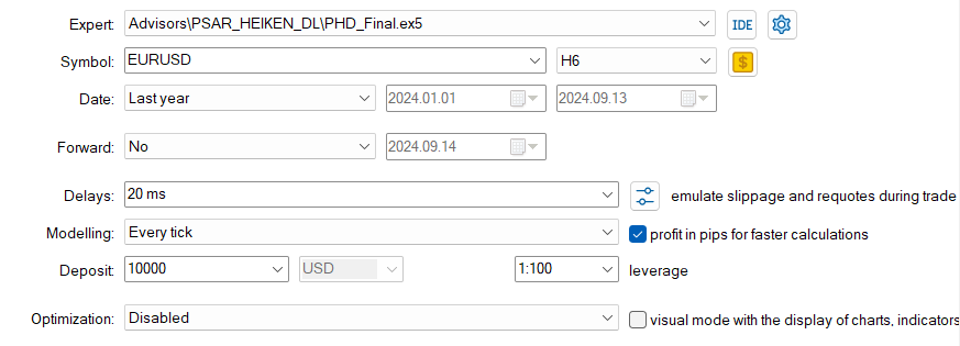
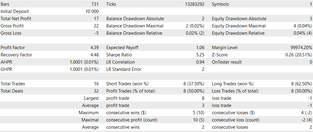
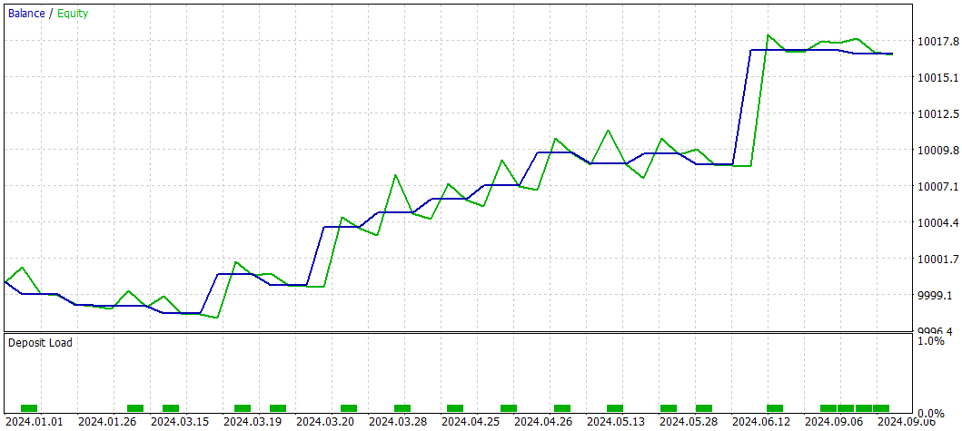
The results of the Expert Advisor (EA) provide an insightful look into its performance during the backtesting period. Starting with an initial deposit of $10,000, the strategy achieved a modest total net profit of 17 units, indicating that while it did generate profits, they were relatively small in proportion to the initial investment. The balance curve reflects this gradual growth, showing a steady, albeit slow, upward trajectory over time.

One of the standout metrics here is the Profit Factor of 4.39. This is a solid number, suggesting that for every unit of risk taken, the strategy earned 4.39 units of reward. It implies that the EA was effective at maximizing profits compared to its losses. The Recovery Factor of 4.48 further supports this, showing that the strategy was able to recover from drawdowns effectively, which is a positive sign for its robustness. However, it’s worth noting the Sharpe Ratio, which sits at 5.25. While this ratio is relatively high and generally indicates good risk-adjusted returns, the overall small profit suggests the strategy might have been taking very minimal risks, leading to the limited absolute profit.

Delving into the trade statistics, the EA executed 16 trades in total, evenly split between long and short positions. The win rate for long trades was higher at 62.5%, while short trades had a win rate of 37.5%. This disparity indicates that the strategy was more successful in capturing upward market movements. Interestingly, the profit trades constituted exactly 50% of the total trades, highlighting that the EA's profitability wasn't due to a high win rate but rather to the size of its winners versus its losers. The largest and average profit trades were both positive, suggesting that the EA managed to secure gains when the market moved favorably. The balance curve reflects these results, showing periods of drawdown followed by gains that indicate a careful but steady approach to trading.

The drawdown metrics show that the EA maintained a low level of risk exposure. The balance drawdown absolute was 2 units, which is quite small, and the drawdown relative was just 0.02%. This very low drawdown suggests that the EA's strategy was conservative, prioritizing capital preservation over aggressive profit-seeking. This conservative approach can be beneficial in volatile markets but also explains the relatively modest total net profit.

In summary, the EA demonstrated a cautious and systematic approach to trading, focusing on maintaining a high profit factor and minimizing drawdowns. While the total profit was relatively small, the high profit factor and low drawdowns indicate a strategy that is more about risk management than rapid profit generation. This makes the EA suitable for traders who prioritize steady, low-risk growth over more aggressive, high-risk strategies. However, for those seeking higher absolute returns, the EA might need further tuning or enhancement to increase its profit potential while maintaining its solid risk management framework.

Conclusion

The exploration of integrating deep learning models with traditional technical analysis has shown promising results. Through the Python script, we’ve seen how a systematic approach using historical data, key indicators, and machine learning can help identify potential trading opportunities. The results were modest yet consistent, demonstrating that such a combination can yield a positive outcome, albeit with some limitations. Similarly, the MetaTrader 5 Expert Advisor (EA) confirmed this cautious approach. While the EA’s performance during backtesting revealed a small but steady growth with minimal drawdown, it highlighted a strategy focused on managing risk rather than maximizing profit. This conservative nature makes it appealing for traders who prioritize steady, low-risk growth. However, for those looking to push for higher returns, further refinement and optimization are needed. In the end, these tools serve as a foundation—a starting point for traders to blend human intuition with the analytical power of AI, offering a nuanced approach to navigating the complex world of forex trading.