Matrix Factorization: A more practical modeling

Introduction

Hello guys and welcome to my new article, which again features didactic content.

In the previous article "Matrix Factorization: The Basics", I talked a little about how you, my dear readers, can use matrices in your general calculations. However, at that time I wanted you to understand how the calculations were done, so I didn't pay much attention to creating the correct model of the matrices.

You might not have noticed that the matrix modeling was a little strange, since only columns were specified, not rows and columns. This looks very strange when reading the code that performs matrix factorizations. If you were expecting to see the rows and columns listed, you might get confused when trying to factorize.

Moreover, this matrix modeling method is not the best. This is because when we model matrices in this way, we encounter some limitations that force us to use other methods or functions that would not be necessary if the modeling were done in a more appropriate way.

Since the procedure, although not complicated, requires a good understanding of it to use it correctly, I chose not to go into detail in the previous article. In this article we will consider everything more calmly, without haste, so as to avoid wrong ideas about modeling matrices to ensure their correct factorization.

Matrices are, by their nature, a better way to perform certain types of computations because they require minimal additional implementation work on our part. However, for exactly the same reason, you should take great care when implementing anything in matrices. Unlike conventional modeling, if we model something incorrectly in matrices, we will get rather strange results or, at best, will face great difficulties in maintaining the developed code.

Care in modeling a matrix

You might wonder why I said the modeling in the previous article was strange, since it all makes sense. Perhaps, you understood everything that was described in that article. Well, let's look at the code fragment from the previous article, in which matrices were modeled. Perhaps this will make it a little clearer what I want to show you. Here is this code.

20. //+------------------------------------------------------------------+
21. void Arrow(const int x, const int y, const ushort angle, const uchar size = 100)
22. {
23.     double M_1[2][2] = {
24.                            cos(_ToRadians(angle)), sin(_ToRadians(angle)),
25.                           -sin(_ToRadians(angle)), cos(_ToRadians(angle))
26.                         },
27.            M_2[][2]  =  {
28.                            0.0,  0.0,
29.                            1.5, -.75,
30.                            1.0,  0.0,
31.                            1.5,  .75
32.                         },
33.            M_3[M_2.Size() / 2][2];

Although it works, as you can see from the fragment, the issue is quite confusing. It's hard to understand. When we write a multidimensional array in code, we use the following configuration:

Label[Dimension_01][Dimension_02]....[Dimension_N];

Although the code may seem simple in general, this type of notation is difficult to understand when applied to the field of matrix factorization. This is because when working with matrices, this way of expressing in a multidimensional array introduces confusion. You will soon understand the reason. To make it simpler, we will reduce this concept to a two-dimensional system, i.e. only to rows and columns. However, matrices can have any number of dimensions. If simplified to a two-dimensional matrix, the notation will look like this:

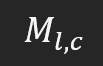
What does this mean? The letter "M" stands for the name of the matrix, "l" stands for the number of rows, and "c" stands for the number of columns. In general, when referring to a matrix element, we will use the same notation, which looks like this:

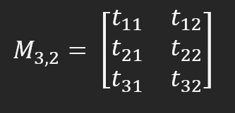
Note that the matrix M now consists of six elements, which can be accessed using the row and column system. But look closely at the previous image: What does it look like? Depending on your experience, it may look different. However, what would this be in programming terminology? So this is a two-dimensional array. But with this approach the matrix appears static. A matrix is a dynamic entity; it can be read in different ways depending on what we are computing. In some cases, we need to read it diagonally, in others column by column, and row by row. Thus, thinking of a matrix as a multidimensional array turns something dynamic into something static. This complicates the implementation of some matrix computations.

However, we are not here to learn the basics of programming. I want to show you, my dear readers, how to best visualize any matrix while allowing it to remain the dynamic entity it is meant to be.

Thus, the idea of a matrix as an array is not incorrect. The problem arises when considering it as a multidimensional array. Ideally, you should think of a matrix as a one-dimensional array, but without a fixed number of dimensions. This point may sound strange, but the problem lies in the language. There are currently no suitable terms or expressions to describe some concepts.

Remember the difficulties Isaac Newton had to face when he first explained his computations. It must have been quite difficult due to the lack of appropriate terms for some concepts. But let's get back to our question.

We already have a way to represent a matrix as an array. But now the first problem arises: How to sort the elements in the array? If you don't understand why this is a problem, then you don't understand other related things concerning matrix factorization. The way the elements are ordered will largely determine how the factorization code is implemented. Although the results are the same in both cases, we may need more or less transitions within the array to get the correct result. This is due to the fact that computer memory is linear. If we order the elements as t11, t12, t21, t22, t31, and t32, which is fine in many cases, we will need to force jumps in order to access the elements in a different order to perform a certain computation. This will certainly happen no matter what we do.

Typically, when we sort elements of an array, we do so by reading line by line. However, you can order them in a different way: for example, reading column by column or in any other way at your discretion. Feel free to do it however you feel comfortable with.

Once this is done, another small problem arises, which is not related to programming but to how matrix factorization is performed. In this case, I will not go into details. The reason is simple: How we deal with this depends on how we implemented the matrix or what kind of matrix we use. I recommend studying books or mathematical literature to understand how to implement solutions to problems that may arise and to perform factorization correctly. However, implementing code is never difficult, because code is the easiest part of the development. The hardest part is to understand how the factorization will be performed. An example is the calculation of the matrix determinant shown in the previous figure. Note that this is not a square matrix, and constructing the determinant in this case is slightly different than what we would do in the case of a square matrix. As already mentioned, it is necessary to study the mathematical part, since each specific case may require a special approach.

A confusion

Well, now that everything is explained, we can move on to the coding stage. Let's continue with the example discussed in the previous article, as it is quite practical and easy to understand. Moreover, this example easily shows another advantage of using matrix computations in some situations. Let's remember what the code looked like. So, here is this code:

01. //+------------------------------------------------------------------+
02. #property copyright "Daniel Jose"
03. #property indicator_chart_window
04. #property indicator_plots 0
05. //+------------------------------------------------------------------+
06. #include <Canvas\Canvas.mqh>
07. //+------------------------------------------------------------------+
08. CCanvas canvas;
09. //+------------------------------------------------------------------+
10. #define _ToRadians(A) (A * (M_PI / 180.0))
11. //+------------------------------------------------------------------+
12. void MatrixA_x_MatrixB(const double &A[][], const double &B[][], double &R[][], const int nDim)
13. {
14.     for (int c = 0, size = (int)(B.Size() / nDim); c < size; c++)
15.     {
16.         R[c][0] = (A[0][0] * B[c][0]) + (A[0][1] * B[c][1]);
17.         R[c][1] = (A[1][0] * B[c][0]) + (A[1][1] * B[c][1]);
18.     }
19. }
20. //+------------------------------------------------------------------+
21. void Arrow(const int x, const int y, const ushort angle, const uchar size = 100)
22. {
23.     double M_1[2][2]{
24.                         cos(_ToRadians(angle)), sin(_ToRadians(angle)),
25.                         -sin(_ToRadians(angle)), cos(_ToRadians(angle))
26.                     },
27.            M_2[][2] {
28.                         0.0,  0.0,
29.                         1.5, -.75,
30.                         1.0,  0.0,
31.                         1.5,  .75
32.                     },
33.            M_3[M_2.Size() / 2][2];
34. 
35.     int dx[M_2.Size() / 2], dy[M_2.Size() / 2];
36.     
37.     MatrixA_x_MatrixB(M_1, M_2, M_3, 2);
38.     ZeroMemory(M_1);
39.     M_1[0][0] = M_1[1][1] = size;
40.     MatrixA_x_MatrixB(M_1, M_3, M_2, 2);
41. 
42.     for (int c = 0; c < (int)M_2.Size() / 2; c++)
43.     {
44.         dx[c] = x + (int) M_2[c][0];
45.         dy[c] = y + (int) M_2[c][1];
46.     }
47. 
48.     canvas.FillPolygon(dx, dy, ColorToARGB(clrPurple, 255));
49.     canvas.FillCircle(x, y, 5, ColorToARGB(clrRed, 255));
50. }
51. //+------------------------------------------------------------------+
52. int OnInit()
53. {    
54.     int px, py;
55.     
56.     px = (int)ChartGetInteger(0, CHART_WIDTH_IN_PIXELS, 0);
57.     py = (int)ChartGetInteger(0, CHART_HEIGHT_IN_PIXELS, 0);
58. 
59.     canvas.CreateBitmapLabel("BL", 0, 0, px, py, COLOR_FORMAT_ARGB_NORMALIZE);
60.     canvas.Erase(ColorToARGB(clrWhite, 255));
61.         
62.     Arrow(px / 2, py / 2, 160);
63. 
64.     canvas.Update(true);
65.     
66.     return INIT_SUCCEEDED;
67. }
68. //+------------------------------------------------------------------+
69. int OnCalculate(const int rates_total, const int prev_calculated, const int begin, const double &price[])
70. {
71.     return rates_total;
72. }
73. //+------------------------------------------------------------------+
74. void OnDeinit(const int reason)
75. {
76.     canvas.Destroy();
77. }
78. //+------------------------------------------------------------------+

Since this code was described in the previous article and is also available in the appendix to it, we will not repeat it here. Let's focus only on the Arrow procedure and the MatrixA_x_MatrixB procedure that actually do something in our demo code.

First, let's change the way arrays are created. The changes will actually be simpler and more subtle than they might seem, but they will still change how we need to get started.

Let's start with the M_1 array shown in the code above. Study it to understand what it is about.

Note that there is something interesting here, which is precisely related to the topic discussed in the previous section. Line 23 declares an array or matrix M_1 with two rows and two columns. In this case, this is quite straightforward. The same applies to an array or matrix M_2, which does not have a definition of the number of rows, but does have a definition of the number of columns, the number of which is equal to two. Up to this point there are no doubts or problems; it is quite easy to understand what we are doing, since each new line in the code corresponds to a new row in the matrix, and each new column in that row will be a new column in the matrix. It's all very simple. However, there is a problem, which lies in the code of the MatrixA_x_MatrixB procedure. Can you identify the problem? No? Or Yes? Perhaps, you may see it but don't understand.

In fact, the problem lies in the MatrixA_x_MatrixB procedure, which is responsible for matrix multiplication. Since what we're doing here is pretty simple, it doesn't interfere with the implementation of the code. However, we still need to solve the problem, because it exists and is slowing down our progress. As soon as we need to implement more complex multiplication, this becomes a real obstacle.

If you didn't notice the problem, pay attention to variable B. It is a matrix that multiplies another matrix. To better visualize the problem, let's reduce matrix B to one column but with two rows, since matrix A has two columns. To perform multiplication, you need to do what is shown in the picture below.

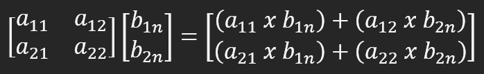
This will give us the correct result. This is exactly what happens when you multiply or factorize a matrix. For more detailed information, I suggest you study this issue. In either case, the multiplication is performed row by row in the column, resulting in the value that remains in the column. This happens because the second factor is a column. If the multiplication is performed in columns, the resulting value must be placed in the form of rows.

Although it seems that all that has been said can only confuse you, in fact this is exactly the rule for performing matrix multiplication. When another programmer analyzes the code, they will not see that everything is done correctly. This is the problem that can be seen in lines 16 and 17, where the calculation shown in the figure above must be performed. But in matrix A we use row-wise calculation, and in matrix B we also use row-wise calculation. This confuses us, although in this simple example it provides the correct data.

You might think: so what? If everything works, leave it as is. But that's not the point. If at some point you need to improve the code to handle a larger matrix or cover a slightly different case, then we'll end up making the problem much more complicated by trying to make something relatively simple work. So such things should be done properly to avoid confusion. To solve this problem, we need to replace this model with a slightly different one. Although it may all seem confusing at first, it will be correct, exactly as shown in the picture above.

To avoid confusion, let's look at how to do this in a new topic.

Making things easier

While what we are going to do here may seem complicated, it really isn't if done correctly and with due care. This might be more tedious, but we will do this in a fairly simple way. Look at the figure below.

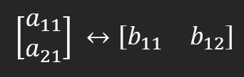
This representation demonstrates that both matrices are equivalent. This is because the matrix with elements A on the left side is a row matrix. When transforming it into a matrix with B elements on the right hand side, which in this case is a column matrix, we don't have to make many changes, maybe just spinning or changing the index in some cases. However, we may need to do this more than once: to transform a row matrix into a column matrix and vice versa, to factorize matrices. But for this example to be correct, a11 must equal b11, and a21 must equal b12.

In some cases, you may notice that there is no need to make any major changes, just a change in the index that will allow us to transform the row structure into one of the columns. But how to do this correctly will depend on each specific case. Therefore, it is important to learn how matrix factorization is done from the relevant math books.

Now let's go back to our code that we looked at in the previous topic. First, let's correct the presentation. Let's change the code as shown below.

20. //+------------------------------------------------------------------+
21. void Arrow(const int x, const int y, const ushort angle, const uchar size = 100)
22. {
23.     double  M_1[]= {
24.                        cos(_ToRadians(angle)), sin(_ToRadians(angle)),
25.                        -sin(_ToRadians(angle)), cos(_ToRadians(angle))
26.                    },
27.             M_2[]= {
28.                        0.0,  0.0,
29.                        1.5, -.75,
30.                        1.0,  0.0,
31.                        1.5,  .75
32.                    },
33.            M_3[M_2.Size()];

Notice that we no longer have indices in the arrays. The matrix structure is created as shown in the code, that is, rows are rows and columns are columns. However, pay attention to dynamic arrays such as M_3. We must define the assigned length correctly to avoid RUN-TIME errors when accessing the elements of these matrices.

This is the first part. After this, the MatrixA_x_MatrixB procedure will no longer be able to understand how to perform calculations. Also, the loop in line 42 (see code in the previous topic) will not be able to decode the data correctly.

First we will correct the calculations performed in the MatrixA_x_MatrixB procedure, and then we will correct the plot. However, before we continue, note that the matrix M_1 is virtually unchanged, as it is symmetrical and square. This is one of the cases where we can read it in both rows and columns.

Since most of the code will change, let's look at the new piece of code. I think this will make it easier to explain how it will all work.

09. //+------------------------------------------------------------------+
10. #define _ToRadians(A) (A * (M_PI / 180.0))
11. //+------------------------------------------------------------------+
12. void MatrixA_x_MatrixB(const double &A[], const ushort Rows, const double &B[], double &R[])
13. {
14.     uint Lines = (uint)(A.Size() / Rows);
15. 
16.     for (uint cbl = 0; cbl < B.Size(); cbl += Rows)
17.         for (uint car = 0; car < Rows; car++)
18.         {
19.             R[car + cbl] = 0;
20.             for (uint cal = 0; cal < Lines; cal++)
21.                 R[car + cbl] += (A[(cal * Rows) + car] * B[cal + cbl]);
22.         }
23. }
24. //+------------------------------------------------------------------+
25. void Plot(const int x, const int y, const double &A[])
26. {
27.     int dx[], dy[];
28. 
29.     for (uint c0 = 0, c1 = 0; c1 < A.Size(); c0++)
30.     {
31.         ArrayResize(dx, c0 + 1, A.Size());
32.         ArrayResize(dy, c0 + 1, A.Size());
33.         dx[c0] = x + (int)(A[c1++]);
34.         dy[c0] = y + (int)(A[c1++]);
35.     }
36. 
37.     canvas.FillPolygon(dx, dy, ColorToARGB(clrPurple, 255));
38.     canvas.FillCircle(x, y, 5, ColorToARGB(clrRed, 255));
39. 
40.     ArrayFree(dx);
41.     ArrayFree(dy);
42. }
43. //+------------------------------------------------------------------+
44. void Arrow(const int x, const int y, const ushort angle, const uchar size = 100)
45. {
46.     double  M_1[]={
47.                      cos(_ToRadians(angle)), sin(_ToRadians(angle)),
48.                      -sin(_ToRadians(angle)), cos(_ToRadians(angle))
49.                   },
50.             M_2[]={
51.                      0.0,  0.0,
52.                      1.5, -.75,
53.                      1.0,  0.0,
54.                      1.5,  .75
55.                   },
56.            M_3[M_2.Size()];
57.     
58.     MatrixA_x_MatrixB(M_1, 2, M_2, M_3);
59.     ZeroMemory(M_1);
60.     M_1[0] = M_1[3] = size;
61.     MatrixA_x_MatrixB(M_1, 2, M_3, M_2);
62.     Plot(x, y, M_2);
63. }
64. //+------------------------------------------------------------------+

It seems like everything has become much more complicated now. Do we really need all this confusion? Calm down my dear reader. This code is neither complicated nor confusing. It is actually very simple and clear. Moreover, it is very flexible. I will explain why I think so.

In this fragment, the multiplication between two matrices is done correctly. In this case, we implemented a column-in-row model, which resulted in a new row being obtained as the product of the multiplication. The multiplication occurs exactly in line 21. I know the procedure performed in line 12 may seem very complicated, but it is not. All these variables exist to ensure correct access to a specific index in the array.

Since there are no tests to ensure that the number of rows in one matrix is equal to the number of columns in the other, we must be careful when using this procedure to avoid RUN-TIME errors.

Now that matrix A, which must be organized in columns, multiplies matrix B, which must be organized in rows, and the result is placed into matrix R, which is organized in rows, we can see how the calls are made. This happens on lines 58 and 61. First, let's look at line 58. The first matrix to be passed is the column matrix M_1. As the second matrix we pass the matrix M_2, which is dynamic and organized by rows. If we change this order in line 58, we will get an error in the calculated values. I know it may seem strange that 2 x 3 is different from 3 x 2, but when it comes to matrices, the order of the factors does affect the outcome. Note, however, that this is similar to what was done before. Of course, the second argument of the call specifies the number of columns in the first matrix. Since our goal here is didactic, I will not check whether it is possible to multiply matrix B (in this case M_2) by matrix A (M_1). I assume that you will not change the structure, perhaps just increase the number of rows in the matrix M_2, which will not affect the factorization in MatrixA_x_MatrixB.

Good. Lines 59 and 60 have already been explained in the previous article, and what happens in line 61 is equivalent to what happens in line 58, so we can assume that the explanation has already been given. However, in line 62 we have a new call that calls the procedure in line 25. Line 25 can be used to plot other objects or images directly on the screen. All we need to do is pass this procedure a row-type matrix, where each row represents a vertex of the image to be drawn. The points that should be in the matrix should be in the following order: X in the first column and Y in the second, since we are plotting on a two-dimensional screen. So even if we are drawing something in 3D, we need to do some calculations in the matrix so that the vertex in the Z dimension is projected onto the XY plane. We don't have to worry about separating things or the size of the matrix. The Plot method will do this. Notice that in line 27 we declare two dynamic arrays. In line 29, we create an interesting for loop that is different from how many people are used to writing loops. In this loop we have two variables: one is controlled by the loop and the other is inside the code. The variable c0 is managed by a loop that tries to correctly instantiate the index for dx and dy and allocates more memory if necessary. This is done in lines 31 and 32. While this may seem inefficient, take a look at the MQL5 documentation and you will see that this is not the case at all.

On the other hand, the variable c1 is managed within the code. To understand this, let's look at what happens to c1 in lines 33 and 34. Each iteration increases by one. However, it is c1 that determines when the for loop should terminate. Look at line 29 for the loop termination condition.

Here we do not check whether the array or matrix A is structured correctly. If we don't have two columns in a row, then at some point in this for loop a RUN-TIME error will be generated, indicating that an attempt was made to access a position that is out of range. Therefore, you should be careful when creating matrix A.

At the end of all this, we use line 37 to call a method from the CCanvas class. This is done in order to plot the matrix shape on the chart. Line 38 shows the location of the point from which the plotting begins. If everything goes well, we will see the image below.

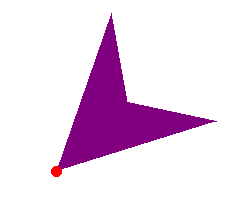
And of course, in lines 40 and 41 we return the allocated memory to the operating system, thus freeing the allocated resource.

Final considerations

In these last two articles, I have tried to cover something that many people find difficult to do: matrix factorization. I know that the material presented here does not cover all the aspects and benefits of using matrices in computations. However, I want to emphasize that it is very important to understand how to develop methods for computing matrices. 3D programs, including games and vector image editors, use this type of factorization. Even seemingly simple programs (such as raster image programs) also use matrix computations to optimize system performance.

In these two articles, I have tried to show this in the simplest way possible because I have noticed that many newcomers to the programming world simply ignore the need to learn certain things. Often they use libraries or other fancy software without realizing what's going on behind the scenes.

Here I tried to simplify the process as much as possible. I focused on one operation: multiplying two matrices. And to demonstrate how simple it is, I didn't show how to use the GPU to do the work that is done in the MatrixA_x_MatrixB procedure, which is what happens in many cases. Here we use only the CPU. But in general, matrix factorization is usually performed not on the CPU, but on the GPU, using OpenCL for correct programming.

I think in a way I have shown that we can do much more than some people think is possible. Study the material presented in the articles, because soon I am going to talk about a topic in which matrix factorization is fundamental.

And the last detail I want to add is that the multiplication of two matrices is aimed at solving a specific problem. This is far from the method that is traditionally taught in books or in school. Don't expect to use this factorization model in general, because it won't work. It is only suitable for solving the proposed problem, which is to rotate an object.