Example of CNA (Causality Network Analysis), SMOC (Stochastic Model Optimal Control) and Nash Game Theory with Deep Learning

Introduction

We are going to walk through the process of adding Deep Learning to three advanced trading Experts Advisors, this three experts are advanced EA's that were published as articles. 

These three articles are published here in www.mql5.com

1. Application of Nash's Game Theory with HMM Filtering in Trading
2. Example of Causality Network Analysis (CNA) and Vector Auto-Regression Model for Market Event Prediction
3. Example of Stochastic Optimization and Optimal Control

If you have not read about this articles, I will explain what are they very briefly, but I strongly recommend reading the articles.

Nash Game Theory

Nash equilibrium is considered one of the basic components of Game theory. 

Nash Equilibrium is a concept in game theory where each player is assumed to know the equilibrium strategies of the other players, and no player has anything to gain by changing only their own strategy.

In a Nash equilibrium, each player's strategy is optimal given the strategies of all other players. A game may have multiple Nash equilibrium or none.

Causality Network Analysis

Causality Network Analysis (CNA) is a method used to understand and model complex causal relationships between variables in a system. When applied to financial markets, it can help identify how different market events and factors influence each other, potentially leading to more accurate predictions.

The bot uses Fast Causality Inference.

Fast casual inference is a concept that combines rapid statistical inference with causal analysis. It aims to draw causal conclusions quickly from data, balancing speed and causal understanding. This approach is useful in scenarios requiring swift, data-driven decisions while also needing insights into cause-effect relationships. Applications may include real-time market analysis, quick business decision-making, and rapid epidemiological studies. The method trades off some depth of analysis for speed, making it suitable for time-sensitive environments where understanding causal links is crucial.

Stochastic Optimization

Stochastic modeling and control optimization are mathematical techniques that help solve problems under conditions of uncertainty. They find application in finance, engineering, artificial intelligence, and many other areas.

Stochastic modeling is used to describe systems with elements of randomness, such as price movements on the stock market or a queue at a restaurant. It is based on random variables, probability distributions, and stochastic processes. Methods such as Monte Carlo and Markov chains can model these processes and predict their behavior.

Management optimization helps you find the best solutions for systems management. It is used to automate and improve the operation of various processes, from driving cars to operating chemical plants. Basic methods include linear quadratic controller, model predictive control, and reinforcement learning.

Deep Learning

Deep learning applied to trading uses artificial neural networks to analyze and predict financial market trends. Here's a brief overview:

1. Data analysis: Deep learning models process vast amounts of financial data, including price histories, trading volumes, economic indicators, and even news sentiment.
2. Pattern recognition: These models can identify complex patterns and relationships in market data that may not be apparent to human traders or traditional analysis methods.
3. Prediction: Based on the patterns identified, deep learning models attempt to predict future market movements, price trends, or optimal trading strategies.
4. Automated trading: Some systems use deep learning to make autonomous trading decisions, executing trades based on the model's predictions.
5. Risk management: Deep learning can be used to assess and manage trading risks more effectively by analyzing multiple risk factors simultaneously.
6. Adaptability: These models can continuously learn and adapt to changing market conditions, potentially improving their performance over time.
7. High-frequency trading: Deep learning can be particularly useful in high-frequency trading scenarios, where split-second decisions are crucial.

While deep learning in trading offers powerful capabilities, it's important to note that markets are complex and unpredictable. These models are not infallible and still require careful oversight and risk management.

Why should we have an EA with Deep Learning?

We will make a Deep Learning model with python, creating a ONNX model, and we will add that model to each of the EA's, and we will compare results with and without Deep Learning.

ONNX models will be used because they can be made easily in python, and they are a bridge for different ecosystems, promoting flexibility and efficiency in model development and deployment. Python is a fast way to make ONNX models or back-testing quickly a strategy. For this article, we will use Python 3.11.9.

We will use Deep Learning with this EA's because the previous results from the articles could be better, we will add conditions for the EA to execute trades or not if the Deep Learning models also say so.

The Python Script

We will use this .py script, this script makes a DL model in ONNX, and also has metrics to see if the model is correctly done, DL has problems when done incorrectly because it can be under fitted or over-fitted, with lead to incorrect predictions.

#python 3.11.9, tensorflow==2.12.0, keras==2.12.0,  tf2onnx==1.16.0
# python libraries
import MetaTrader5 as mt5
import tensorflow as tf
import numpy as np
import pandas as pd
import tf2onnx
#import tensorflow as tf
#import tf2onnx
import keras

print(f"TensorFlow version: {tf.__version__}")
print(f"Keras version: {keras.__version__}")
print(f"tf2onnx version: {tf2onnx.__version__}")


# input parameters

inp_history_size = 120

sample_size = inp_history_size*3*20
symbol = "EURUSD"
optional = "D1_2024"
inp_model_name = str(symbol)+"_"+str(optional)+".onnx" 

if not mt5.initialize():
    print("initialize() failed, error code =",mt5.last_error())
    quit()

# we will save generated onnx-file near the our script to use as resource
from sys import argv
data_path=argv[0]
last_index=data_path.rfind("\\")+1
data_path=data_path[0:last_index]
print("data path to save onnx model",data_path)

# and save to MQL5\Files folder to use as file
terminal_info=mt5.terminal_info()
file_path=terminal_info.data_path+"\\MQL5\\Files\\"
print("file path to save onnx model",file_path)

# set start and end dates for history data
from datetime import timedelta, datetime
#end_date = datetime.now()
end_date = datetime(2024, 1, 1, 0)
start_date = end_date - timedelta(days=inp_history_size*20)

# print start and end dates
print("data start date =",start_date)
print("data end date =",end_date)

# get rates
eurusd_rates = mt5.copy_rates_from(symbol, mt5.TIMEFRAME_D1, end_date, sample_size)

# create dataframe
df = pd.DataFrame(eurusd_rates)

# get close prices only
data = df.filter(['close']).values

# scale data
from sklearn.preprocessing import MinMaxScaler
scaler=MinMaxScaler(feature_range=(0,1))
scaled_data = scaler.fit_transform(data)

# training size is 80% of the data
training_size = int(len(scaled_data)*0.80) 
print("Training_size:",training_size)
train_data_initial = scaled_data[0:training_size,:]
test_data_initial = scaled_data[training_size:,:1]

# split a univariate sequence into samples
def split_sequence(sequence, n_steps):
    X, y = list(), list()
    for i in range(len(sequence)):
       # find the end of this pattern
       end_ix = i + n_steps
       # check if we are beyond the sequence
       if end_ix > len(sequence)-1:
          break
       # gather input and output parts of the pattern
       seq_x, seq_y = sequence[i:end_ix], sequence[end_ix]
       X.append(seq_x)
       y.append(seq_y)
    return np.array(X), np.array(y)

# split into samples
time_step = inp_history_size
x_train, y_train = split_sequence(train_data_initial, time_step)
x_test, y_test = split_sequence(test_data_initial, time_step)

# reshape input to be [samples, time steps, features] which is required for LSTM
x_train =x_train.reshape(x_train.shape[0],x_train.shape[1],1)
x_test = x_test.reshape(x_test.shape[0],x_test.shape[1],1)



# define model
from keras.models import Sequential
from keras.layers import Dense, Activation, Conv1D, MaxPooling1D, Dropout, Flatten, LSTM
from keras.metrics import RootMeanSquaredError as rmse
from tensorflow.keras import callbacks
model = Sequential()
model.add(Conv1D(filters=256, kernel_size=2, strides=1, padding='same', activation='relu', input_shape=(inp_history_size,1)))
model.add(MaxPooling1D(pool_size=2))
model.add(LSTM(100, return_sequences = True))
model.add(Dropout(0.3))
model.add(LSTM(100, return_sequences = False))
model.add(Dropout(0.3))
model.add(Dense(units=1, activation = 'sigmoid'))
model.compile(optimizer='adam', loss= 'mse' , metrics = [rmse()])

# Set up early stopping
early_stopping = callbacks.EarlyStopping(
    monitor='val_loss',
    patience=20,
    restore_best_weights=True,
)

# model training for 300 epochs
history = model.fit(x_train, y_train, epochs = 300 , validation_data = (x_test,y_test), batch_size=32, callbacks=[early_stopping], verbose=2)

# evaluate training data
train_loss, train_rmse = model.evaluate(x_train,y_train, batch_size = 32)
print(f"train_loss={train_loss:.3f}")
print(f"train_rmse={train_rmse:.3f}")

# evaluate testing data
test_loss, test_rmse = model.evaluate(x_test,y_test, batch_size = 32)
print(f"test_loss={test_loss:.3f}")
print(f"test_rmse={test_rmse:.3f}")

# Define a function that represents your model
@tf.function(input_signature=[tf.TensorSpec([None, inp_history_size, 1], tf.float32)])
def model_function(x):
    return model(x)

output_path = data_path+inp_model_name
# Convert the model to ONNX
onnx_model, _ = tf2onnx.convert.from_function(
    model_function, 
    input_signature=[tf.TensorSpec([None, inp_history_size, 1], tf.float32)],
    opset=13,
    output_path=output_path
)

print(f"Saved ONNX model to {output_path}")


# save model to ONNX
output_path = data_path+inp_model_name
onnx_model = tf2onnx.convert.from_keras(model, output_path=output_path)
print(f"saved model to {output_path}")

output_path = file_path+inp_model_name
onnx_model = tf2onnx.convert.from_keras(model, output_path=output_path)
print(f"saved model to {output_path}")

#prediction using testing data
test_predict = model.predict(x_test)
print(test_predict)
print("longitud total de la prediccion: ", len(test_predict))
print("longitud total del sample: ", sample_size)

plot_y_test = np.array(y_test).reshape(-1, 1)  # Selecciona solo el último elemento de cada muestra de prueba
plot_y_train = y_train.reshape(-1,1)
train_predict = model.predict(x_train)
#print(plot_y_test)

#calculate metrics
from sklearn import metrics
from sklearn.metrics import r2_score
#transform data to real values
value1=scaler.inverse_transform(plot_y_test)
#print(value1)
# Escala las predicciones inversas al transformarlas a la escala original
value2 = scaler.inverse_transform(test_predict.reshape(-1, 1))
#print(value2)
#calc score
score = np.sqrt(metrics.mean_squared_error(value1,value2))

print("RMSE         : {}".format(score))
print("MSE          :", metrics.mean_squared_error(value1,value2))
print("R2 score     :",metrics.r2_score(value1,value2))


#sumarize model
model.summary()

#Print error
value11=pd.DataFrame(value1)
value22=pd.DataFrame(value2)
#print(value11)
#print(value22)



value111=value11.iloc[:,:]
value222=value22.iloc[:,:]

print("longitud salida (tandas de 1 hora): ",len(value111) )
print("en horas son " + str((len(value111))*60*24)+ " minutos")
print("en horas son " + str(((len(value111)))*60*24/60)+ " horas")
print("en horas son " + str(((len(value111)))*60*24/60/24)+ " dias")


# Calculate error
error = value111 - value222

import matplotlib.pyplot as plt
# Plot error
plt.figure(figsize=(7, 6))
plt.scatter(range(len(error)), error, color='blue', label='Error')
plt.axhline(y=0, color='red', linestyle='--', linewidth=1)  # Línea horizontal en y=0
plt.title('Error de Predicción ' + str(symbol))
plt.xlabel('Índice de la muestra')
plt.ylabel('Error')
plt.legend()
plt.grid(True)
plt.savefig(str(symbol)+str(optional)+'.png') 

rmse_ = format(score)
mse_ = metrics.mean_squared_error(value1,value2)
r2_ = metrics.r2_score(value1,value2)

resultados= [rmse_,mse_,r2_]

# Abre un archivo en modo escritura
with open(str(symbol)+str(optional)+"results.txt", "w") as archivo:
    # Escribe cada resultado en una línea separada
    for resultado in resultados:
        archivo.write(str(resultado) + "\n")

# finish
mt5.shutdown()

#show iteration-rmse graph for training and validation
plt.figure(figsize = (7,10))
plt.plot(history.history['root_mean_squared_error'],label='Training RMSE',color='b')
plt.plot(history.history['val_root_mean_squared_error'],label='Validation-RMSE',color='g')
plt.xlabel("Iteration")
plt.ylabel("RMSE")
plt.title("RMSE" + str(symbol))
plt.legend()
plt.savefig(str(symbol)+str(optional)+'1.png') 

#show iteration-loss graph for training and validation
plt.figure(figsize = (7,10))
plt.plot(history.history['loss'],label='Training Loss',color='b')
plt.plot(history.history['val_loss'],label='Validation-loss',color='g')
plt.xlabel("Iteration")
plt.ylabel("Loss")
plt.title("LOSS" + str(symbol))
plt.legend()
plt.savefig(str(symbol)+str(optional)+'2.png') 

#show actual vs predicted (training) graph
plt.figure(figsize=(7,10))
plt.plot(scaler.inverse_transform(plot_y_train),color = 'b', label = 'Original')
plt.plot(scaler.inverse_transform(train_predict),color='red', label = 'Predicted')
plt.title("Prediction Graph Using Training Data" + str(symbol))
plt.xlabel("Hours")
plt.ylabel("Price")
plt.legend()
plt.savefig(str(symbol)+str(optional)+'3.png') 

#show actual vs predicted (testing) graph
plt.figure(figsize=(7,10))
plt.plot(scaler.inverse_transform(plot_y_test),color = 'b',  label = 'Original')
plt.plot(scaler.inverse_transform(test_predict),color='g', label = 'Predicted')
plt.title("Prediction Graph Using Testing Data" + str(symbol))
plt.xlabel("Hours")
plt.ylabel("Price")
plt.legend()
plt.savefig(str(symbol)+str(optional)+'4.png') 

The output this .py script gives looks similar to this:

177/177 - 51s - loss: 2.4565e-04 - root_mean_squared_error: 0.0157 - val_loss: 4.8860e-05 - val_root_mean_squared_error: 0.0070 - 51s/epoch - 291ms/step
177/177 [==============================] - 15s 82ms/step - loss: 1.0720e-04 - root_mean_squared_error: 0.0104
train_loss=0.000
train_rmse=0.010
42/42 [==============================] - 3s 74ms/step - loss: 4.4485e-05 - root_mean_squared_error: 0.0067
test_loss=0.000
test_rmse=0.007
Saved ONNX model to c:\XXXXXXXXXXXXXXX\EURUSD_D1_2024.onnx
saved model to c:\XXXXXXXXXXXXXXXX\EURUSD_D1_2024.onnx
saved model to C:\XXXXXXXXXX\MQL5\Files\EURUSD_D1_2024.onnx
42/42 [==============================] - 5s 80ms/step
[[0.40353602]
 [0.39568084]
 [0.39963558]
 ...
 [0.35914657]
 [0.3671721 ]
 [0.3618655 ]]
longitud total de la prediccion:  1320
longitud total del sample:  7200
177/177 [==============================] - 13s 72ms/step
RMSE         : 0.005155711558172936
MSE          : 2.6581361671078003e-05
R2 score     : 0.9915315181564703
Model: "sequential"
_________________________________________________________________
 Layer (type)                Output Shape              Param #
=================================================================
 conv1d (Conv1D)             (None, 120, 256)          768

 max_pooling1d (MaxPooling1D  (None, 60, 256)          0
 )

 lstm (LSTM)                 (None, 60, 100)           142800

 dropout (Dropout)           (None, 60, 100)           0

 lstm_1 (LSTM)               (None, 100)               80400

 dropout_1 (Dropout)         (None, 100)               0

 dense (Dense)               (None, 1)                 101

=================================================================
Total params: 224,069
Trainable params: 224,069
Non-trainable params: 0
________________________________________________________________

This model might be over-fitted, because of this results, this could be the in the limit of a good prediction and being over-fitted:

RMSE         : 0.005155711558172936
MSE          : 2.6581361671078003e-05
R2 score     : 0.9915315181564703

The principal metrics are this three, R2, gives a percentage of results tested of good predictions, and RMSE, MSE are the errors, if you want to know more about this, you can google it.

As we are going to do this for the same symbol (EURUSD), we only have to make one DL model, and we will test it for 2024.

We have selected the time period time frame of 1 day, to not consume too much of/with our computers.

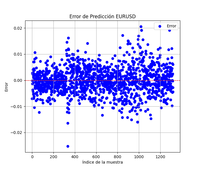
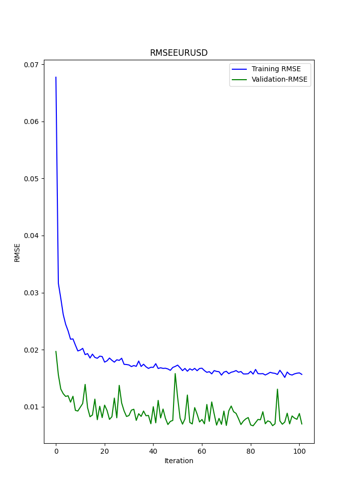
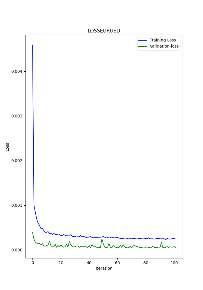
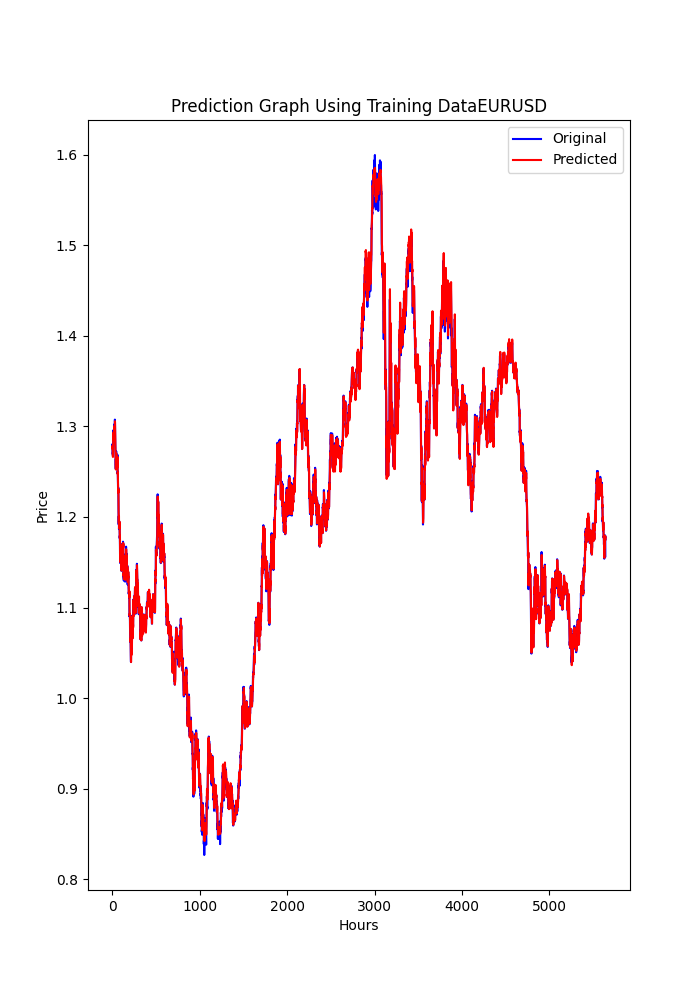
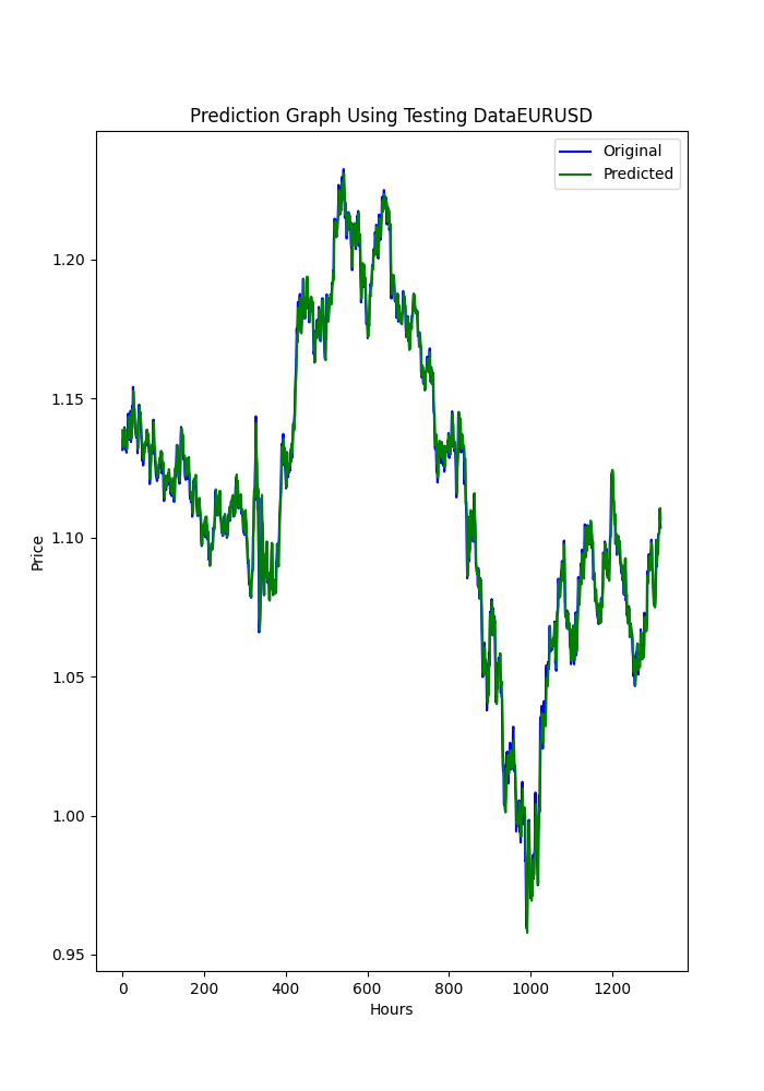
The py script also shows some graphs that are saved (it's another way to see if models are or aren't over or under fitted).

Graphs should look like this:

The script also saves a .txt where the metrics from before are saved in the same order as it appears in the terminal.

To use this script, you must first install Python 3.11.9, and install this libraries with; pip install:

tensorflow==2.12.0, keras==2.12.0,  tf2onnx==1.16.0, MetaTrader5, pandas, numpy, scikit-learn, tf2onnx, keras

I strongly recommend to use Visual Studio Code, that you can download from Microsoft's Store.

It might ask you to install

Microsoft Visual C++ 2015 - 2022 Redistributable

I have attached the .py script, just open it in VSC and run it.

If you want to change anything (another symbol, period from where to get the data or time period), change only this lines:

symbol = "EURUSD"
optional = "D1_2024"

The symbol is obvious, I recommend to change optional to the time period used and the last date of the data.

eurusd_rates = mt5.copy_rates_from(symbol, mt5.TIMEFRAME_D1, end_date, sample_size)

In this line, is where you change the time frame, for example H1 (1 hour time frame).

Now we have the Deep Learning ONNX model, we can add it to the EA's we already have from the other articles.

I will attach the DL ONNX model (2024).

What will we add to the EA's?

CNA Modifications

This is basic, I will go through this process very slowly.

1st, at the beginning, where the inputs parameters, we have to add this lines:

#include <Trade\Trade.mqh>

#resource "/Files/EURUSD_D1.onnx" as uchar ExtModel[]

#define SAMPLE_SIZE 120

long     ExtHandle=INVALID_HANDLE;
int      ExtPredictedClass=-1;
datetime ExtNextBar=0;
datetime ExtNextDay=0;
float    ExtMin=0.0;
float    ExtMax=0.0;
CTrade   ExtTrade;
int dlsignal=-1;

//--- price movement prediction
#define PRICE_UP   0
#define PRICE_SAME 1
#define PRICE_DOWN 2

Remember to modify this line with the ONNX model you made (the py scripts save in MQL5/Files/ ... the model).

#resource "/Files/EURUSD_D1_2024.onnx" as uchar ExtModel[]

On the OnInit() you have to add this:

//--- create a model from static buffer
   ExtHandle=OnnxCreateFromBuffer(ExtModel,ONNX_DEFAULT);
   if(ExtHandle==INVALID_HANDLE)
     {
      Print("OnnxCreateFromBuffer error ",GetLastError());
      return(INIT_FAILED);
     }

//--- since not all sizes defined in the input tensor we must set them explicitly
//--- first index - batch size, second index - series size, third index - number of series (only Close)
   const long input_shape[] = {1,SAMPLE_SIZE,1};
   if(!OnnxSetInputShape(ExtHandle,ONNX_DEFAULT,input_shape))
     {
      Print("OnnxSetInputShape error ",GetLastError());
      return(INIT_FAILED);
     }

//--- since not all sizes defined in the output tensor we must set them explicitly
//--- first index - batch size, must match the batch size of the input tensor
//--- second index - number of predicted prices (we only predict Close)
   const long output_shape[] = {1,1};
   if(!OnnxSetOutputShape(ExtHandle,0,output_shape))
     {
      Print("OnnxSetOutputShape error ",GetLastError());
      return(INIT_FAILED);
     }

Where? Anywhere ... it doesn't matter (just before the function return).

On the OnDeinit function, you must also add this:

if(ExtHandle!=INVALID_HANDLE)
     {
      OnnxRelease(ExtHandle);
      ExtHandle=INVALID_HANDLE;
     }

Where? Anywhere, this releases the ONNX model.

On the OnTick function you must add this:

void OnTick()
  {
  //--- check new day
   if(TimeCurrent()>=ExtNextDay)
     {
      GetMinMax();
      //--- set next day time
      ExtNextDay=TimeCurrent();
      ExtNextDay-=ExtNextDay%PeriodSeconds(PERIOD_D1);
      ExtNextDay+=PeriodSeconds(PERIOD_D1);
     }

//--- check new bar
   if(TimeCurrent()<ExtNextBar)
      return;
//--- set next bar time
   ExtNextBar=TimeCurrent();
   ExtNextBar-=ExtNextBar%PeriodSeconds();
   ExtNextBar+=PeriodSeconds();
//--- check min and max
   float close=(float)iClose(_Symbol,_Period,0);
   if(ExtMin>close)
      ExtMin=close;
   if(ExtMax<close)
      ExtMax=close;
      
   PredictPrice();

Where? At the beginning, this is important because the result of the function PredictPrice(), must be added to the execute order logic.

In OnTick() function, you must also modify the function that makes the orders, in this case (CNA_DL), we will change the original line:

int signal = GenerateSignal(symbol, prediction);

to this line:

int signal = GenerateSignal(symbol, prediction, ExtPredictedClass);

ExtPredictedClass is the result of the PredictedPrice() function we added before.

Now, we also have to modify the logic of GenerateSignal(), so it uses the ExtPredictedClass:

We will have to change the header of that function:

int GenerateSignal(string symbol, double prediction, int dlsgnl)

and add the new variable to the logic to make orders, in this case, here:

from this:

   bool buy_condition =  prediction >  0.00001 && rsi < 30 && trend_strong  && volatility_ok && fastMA > slowMA;
   bool sell_condition = prediction < -0.00001 && rsi > 70 && trend_strong && volatility_ok && fastMA < slowMA;

to this:

   bool buy_condition =  prediction >  0.00001 && rsi < 30 && trend_strong  && volatility_ok && fastMA > slowMA && dlsgnl==PRICE_UP;
   bool sell_condition = prediction < -0.00001 && rsi > 70 && trend_strong && volatility_ok && fastMA < slowMA && dlsgnl==PRICE_DOWN;

The last part we need to modify is this;

We have to add this functions to the script, where? Anywhere, at the end, for example.

//+------------------------------------------------------------------+
void PredictPrice(void)
  {
   static vectorf output_data(1);            // vector to get result
   static vectorf x_norm(SAMPLE_SIZE);       // vector for prices normalize

//--- check for normalization possibility
   if(ExtMin>=ExtMax)
     {
      Print("ExtMin>=ExtMax");
      ExtPredictedClass=-1;
      return;
     }
//--- request last bars
   if(!x_norm.CopyRates(_Symbol,_Period,COPY_RATES_CLOSE,1,SAMPLE_SIZE))
     {
      Print("CopyRates ",x_norm.Size());
      ExtPredictedClass=-1;
      return;
     }
   float last_close=x_norm[SAMPLE_SIZE-1];
//--- normalize prices
   x_norm-=ExtMin;
   x_norm/=(ExtMax-ExtMin);
//--- run the inference
   if(!OnnxRun(ExtHandle,ONNX_NO_CONVERSION,x_norm,output_data))
     {
      Print("OnnxRun");
      ExtPredictedClass=-1;
      return;
     }
//--- denormalize the price from the output value
   float predicted=output_data[0]*(ExtMax-ExtMin)+ExtMin;
//--- classify predicted price movement
   float delta=last_close-predicted;
   if(fabs(delta)<=0.00001)
      ExtPredictedClass=PRICE_SAME;
   else
     {
      if(delta<0)
         ExtPredictedClass=PRICE_UP;
      else
         ExtPredictedClass=PRICE_DOWN;
     }
  }
  
  
  
  void GetMinMax(void)
  {
   vectorf close;
   close.CopyRates(_Symbol,PERIOD_D1,COPY_RATES_CLOSE,0,SAMPLE_SIZE);
   ExtMin=close.Min();
   ExtMax=close.Max();
  }

These two functions are key for predictions, one makes the predictions, and the other get the min and max close.

Modifications in SMOC

Everything stays the same, and the changes are equal to the ones before except for this ones:

In the input parameters you don't initialize dlsignal or add CTrade:

#resource "/Files/EURUSD_D1.onnx" as uchar ExtModel[]

#define SAMPLE_SIZE 120

long     ExtHandle=INVALID_HANDLE;
int      ExtPredictedClass=-1;
datetime ExtNextBar=0;
datetime ExtNextDay=0;
float    ExtMin=0.0;
float    ExtMax=0.0;

//--- price movement prediction
#define PRICE_UP   0
#define PRICE_SAME 1
#define PRICE_DOWN 2

In OnTick(), we will have this:

void OnTick()
  {
//--- check new day
   if(TimeCurrent()>=ExtNextDay)
     {
      GetMinMax();
      //--- set next day time
      ExtNextDay=TimeCurrent();
      ExtNextDay-=ExtNextDay%PeriodSeconds(PERIOD_D1);
      ExtNextDay+=PeriodSeconds(PERIOD_D1);
     }

//--- check new bar
   if(TimeCurrent()<ExtNextBar)
      return;
//--- set next bar time
   ExtNextBar=TimeCurrent();
   ExtNextBar-=ExtNextBar%PeriodSeconds();
   ExtNextBar+=PeriodSeconds();
//--- check min and max
   float close=(float)iClose(_Symbol,_Period,0);
   if(ExtMin>close)
      ExtMin=close;
   if(ExtMax<close)
      ExtMax=close;

   PredictPrice();

   static datetime lastBarTime = 0;
   datetime currentBarTime = iTime(Symbol(), PERIOD_CURRENT, 0);

// Only process on new bar
   if(currentBarTime == lastBarTime)
      return;

   lastBarTime = currentBarTime;

   double currentPrice = SymbolInfoDouble(Symbol(), SYMBOL_LAST);
   int decision = OptimalControl(currentPrice);

   string logMessage = StringFormat("New bar: Time=%s, Price=%f, Decision=%d",
                                    TimeToString(currentBarTime), currentPrice, decision);
   LogMessage(logMessage);

// Manage open order if exists
   if(orderTicket != 0)
     {
      ManageOpenOrder(decision, ExtPredictedClass);
     }

   if(orderTicket == 0 && decision != 0 && IsTrendFavorable(decision) && IsLongTermTrendFavorable(decision) && (ExtPredictedClass==PRICE_DOWN || ExtPredictedClass==PRICE_UP))
     {
      ExecuteTrade(decision, ExtPredictedClass);
     }
  }

In ManageOpenOrder() we will make this change:

void ManageOpenOrder(int decision, int dlsignal)
  {
   int barsOpen = iBars(Symbol(), PERIOD_CURRENT) - iBarShift(Symbol(), PERIOD_CURRENT, orderOpenTime);
   LogMessage(StringFormat("Bars open: %d for order ticket: %d", barsOpen, orderTicket));

   if(barsOpen >= maxBarsOpen ||
      (PositionGetInteger(POSITION_TYPE) == POSITION_TYPE_BUY && decision == -1 && dlsignal == PRICE_DOWN) ||
      (PositionGetInteger(POSITION_TYPE) == POSITION_TYPE_SELL && decision == 1 && dlsignal == PRICE_UP))
     {
      CloseOrder(orderTicket);
      orderTicket = 0;
      orderOpenTime = 0;
     }
   else
     {
      UpdateSLTP(orderTicket, decision);
     }
  }

In ExecuteTrade()

void ExecuteTrade(int decision, int dlsignal)
  {
   MqlTradeRequest request = {};
   MqlTradeResult result = {};
   double price;
   int decision1;
   
   

   if(decision == 1 && dlsignal == PRICE_UP)
     {
      price = SymbolInfoDouble(Symbol(), SYMBOL_ASK);
      request.type = ORDER_TYPE_BUY;
      decision1 = 1;
     }
   else
      if(decision == -1 && dlsignal == PRICE_DOWN)
        {
         price = SymbolInfoDouble(Symbol(), SYMBOL_BID);
         request.type = ORDER_TYPE_SELL;
        decision1 = -1;
        }
   double sl = CalculateDynamicSL(price, decision1);
   double tp = CalculateDynamicTP(price, decision1);



   double adjustedLotSize = AdjustLotSizeForDrawdown();
   request.volume = adjustedLotSize;

   request.action = TRADE_ACTION_DEAL;
   request.symbol = Symbol();
//request.volume = lotSize;
//request.type = (decision == 1 && dlsignal == PRICE_UP) ? ORDER_TYPE_BUY : ORDER_TYPE_SELL;
   request.price = price;
   request.sl = sl;
   request.tp = tp;
   request.deviation = 10;
   request.magic = 123456; // Magic number to identify orders from this EA
   request.comment = (decision == 1) ? "Buy Order" : "Sell Order";

   if(OrderSend(request, result))
     {
      Print((decision1 == 1 ? "Buy" : "Sell"), " Order Executed Successfully. Ticket: ", result.order);
      orderOpenTime = iTime(Symbol(), PERIOD_CURRENT, 0);
      orderTicket = result.order;
     }
   else
     {
      Print("Error executing Order: ", GetLastError());
     }
  }

And now the modifications on the Nash equity script.

Modifications in Nash Equity

All the changes are the same, except for the OnTick() function, that will be like this one:

void OnTick()
  {
//--- check new day
   if(TimeCurrent()>=ExtNextDay)
     {
      GetMinMax();
      //--- set next day time
      ExtNextDay=TimeCurrent();
      ExtNextDay-=ExtNextDay%PeriodSeconds(PERIOD_D1);
      ExtNextDay+=PeriodSeconds(PERIOD_D1);
     }

//--- check new bar
   if(TimeCurrent()<ExtNextBar)
      return;
//--- set next bar time
   ExtNextBar=TimeCurrent();
   ExtNextBar-=ExtNextBar%PeriodSeconds();
   ExtNextBar+=PeriodSeconds();
//--- check min and max
   float close=(float)iClose(_Symbol,_Period,0);
   if(ExtMin>close)
      ExtMin=close;
   if(ExtMax<close)
      ExtMax=close;

   PredictPrice();

   if(!IsNewBar())
      return; // Solo procesar en nueva barra

   MarketRegime hmmRegime = NOT_PRESENT;
   MarketRegime logLikelihoodRegime = NOT_PRESENT;
   DetectMarketRegime(hmmRegime, logLikelihoodRegime);

// Calcular señales para cada estrategia
   CalculateStrategySignals(_Symbol, TimeCurrent(), hmmRegime, logLikelihoodRegime);

// Verificar si la estrategia de Nash Equilibrium ha generado una señal
   if(strategies[3].enabled && strategies[3].signal != 0)
     {
      if(strategies[3].signal > 0 && ExtPredictedClass==PRICE_UP)
        {
         OpenBuyOrder(strategies[3].name);
        }
      else
         if(strategies[3].signal < 0 && ExtPredictedClass==PRICE_DOWN)
           {
            OpenSellOrder(strategies[3].name);
           }
     }

// Actualizar stops de seguimiento si es necesario
   if(UseTrailingStop)
     {
      UpdateTrailingStops();
     }
  }

Results
CNA_DL

Settings

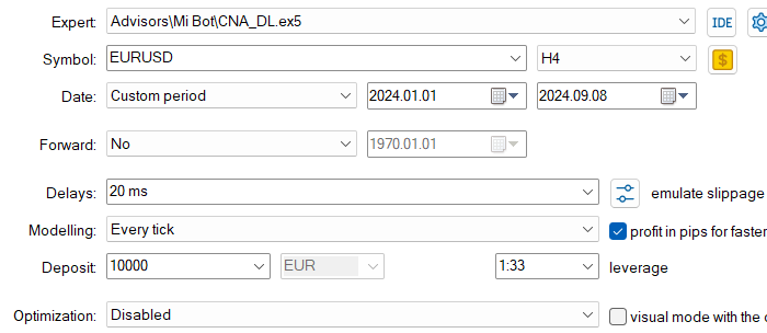
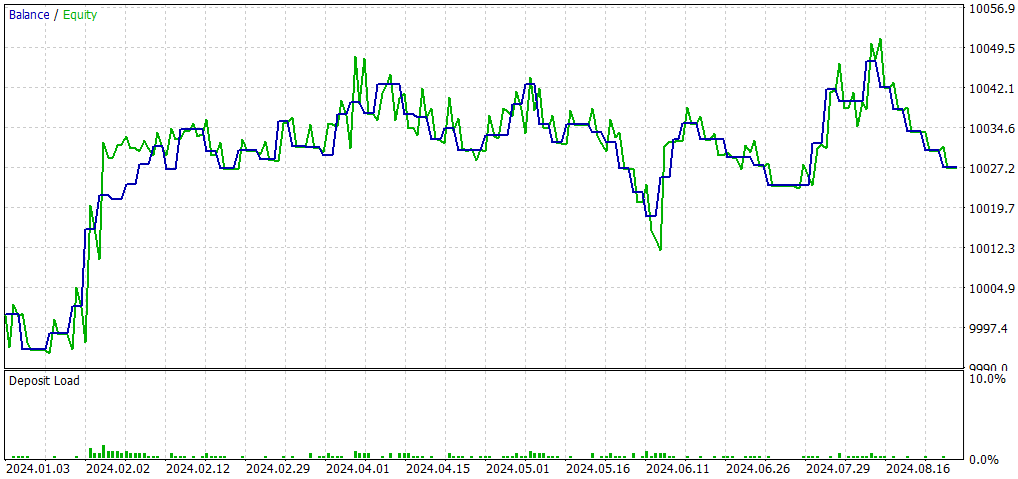
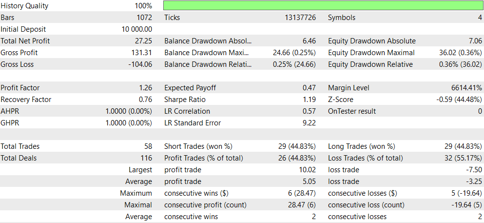
Compared with the original EA (CNA_Final_v4):

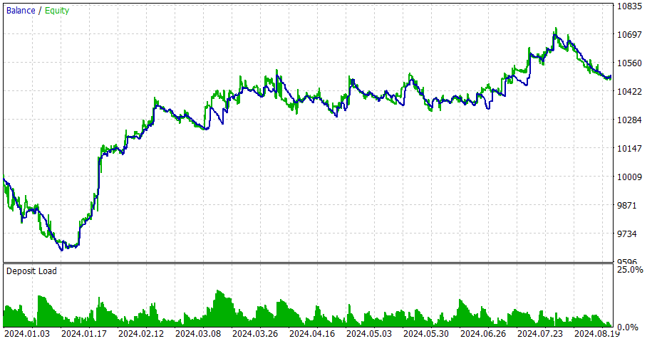
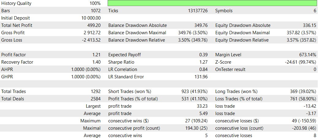
Comparison of CNA with and without Deep Learning

1. Profitability: The non-deep learning EA is significantly more profitable, but it also takes on more risk with higher draw-downs.
2. Risk: The deep learning EA has lower draw-downs and seems more conservative in its approach.
3. Trading Frequency: The non-deep learning EA trades much more frequently (1292 vs 58 trades).
4. Win Rate: The deep learning EA has a slightly better win rate, but both are below 50%.
5. Strategy Bias: The non-deep learning EA shows a strong preference for short trades, while the deep learning EA is balanced.
6. Consistency: The deep learning EA seems more consistent with smaller strings of consecutive wins/losses.

In conclusion, the non-deep learning EA appears to be more profitable but riskier, while the deep learning EA is more conservative with lower returns but also lower risk. The choice between them would depend on the trader's risk tolerance and investment goals. The deep learning EA might be preferred for more stable, conservative trading, while the non-deep learning EA could be chosen for potentially higher returns at the cost of higher risk.

SMOC_DL

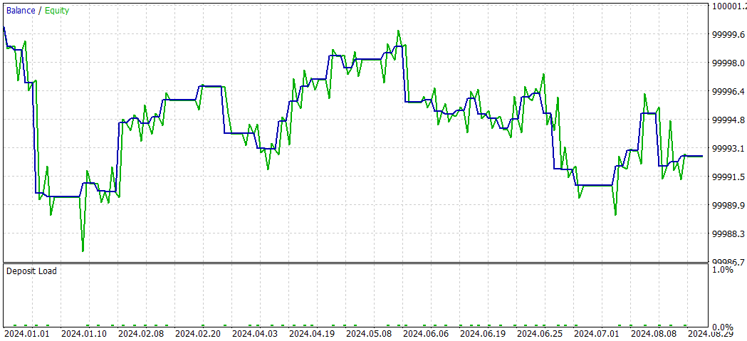
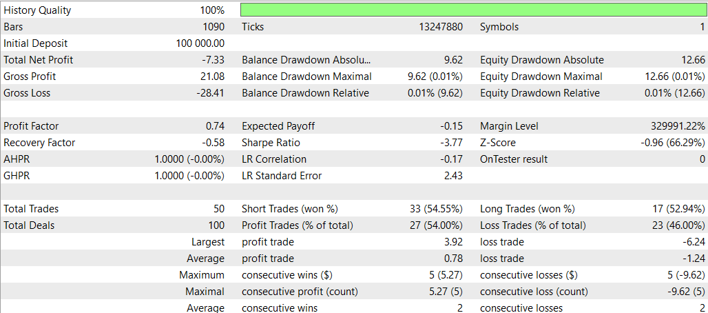
And now SMOC without Deep Learning

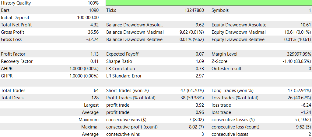
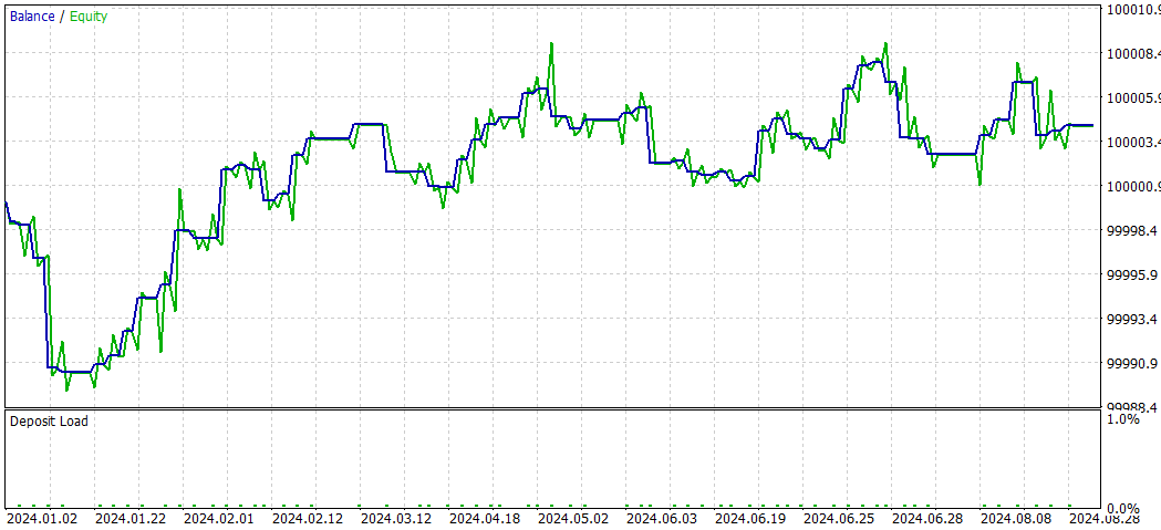
Comparison SMOC_DL vs SMOC:

1. Profitability: Strategy 2 is profitable (4.32), while Strategy 1 is unprofitable (-7.33).
2. Risk-adjusted returns: Strategy 2 has a positive Sharpe Ratio (1.69), indicating better risk-adjusted returns compared to Strategy 1's negative Sharpe Ratio (-3.77).
3. Win rate: Strategy 2 has a higher win rate (59.38%) compared to Strategy 1 (54%).
4. Number of trades: Strategy 2 executes more trades (64) than Strategy 1 (50), potentially indicating more opportunities identified.
5. Profit Factor: Strategy 2 has a profit factor above 1 (1.13), while Strategy 1 is below 1 (0.74), suggesting Strategy 2 is more effective at generating profits relative to losses.
6. Draw-down: Both strategies have similar low draw-downs (0.01% of the account), indicating good risk management.
7. Trade distribution: Both strategies have a preference for short trades, but Strategy 2 has a more balanced distribution between short and long trades.

Overall, Strategy 2 appears to be superior in most aspects, including profitability, risk-adjusted returns, win rate, and profit factor. It also takes more trades, potentially indicating better opportunity identification. Both strategies demonstrate good risk management with low draw-downs. Based on this data, Strategy 2 would be the preferred choice between the two. A suitable approach to use DL would be trying other time frames.

NASH_DL

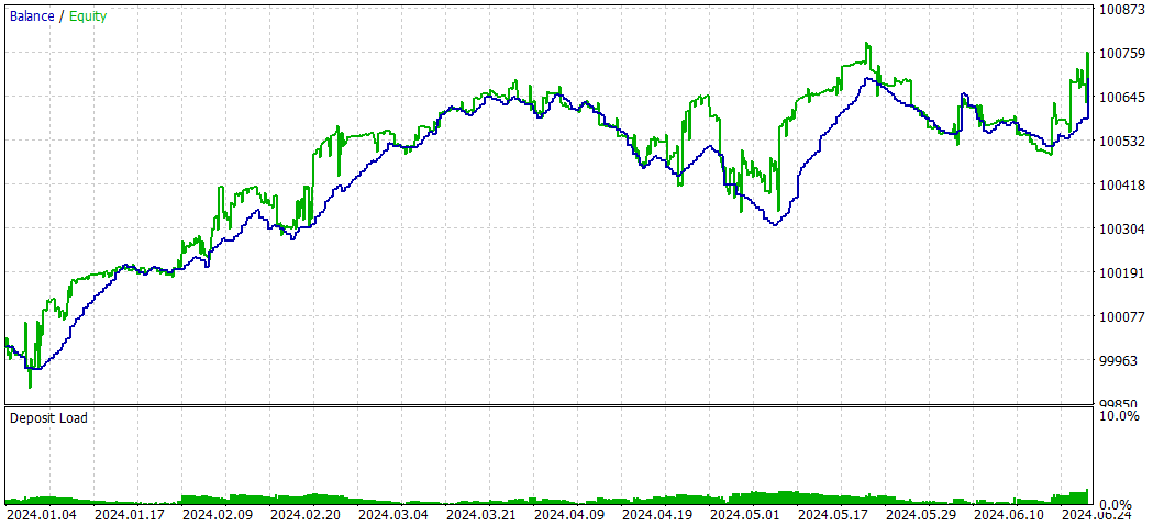
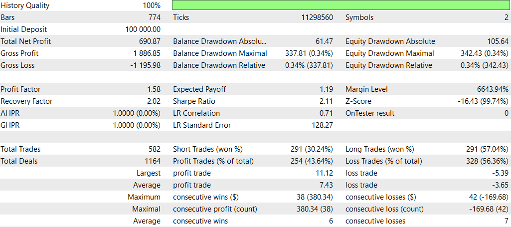
And now without Deep Learning:

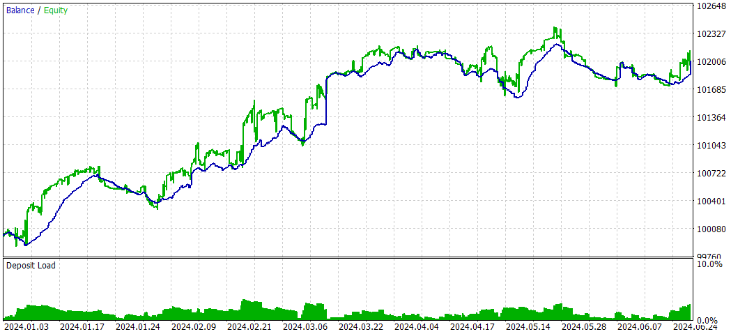
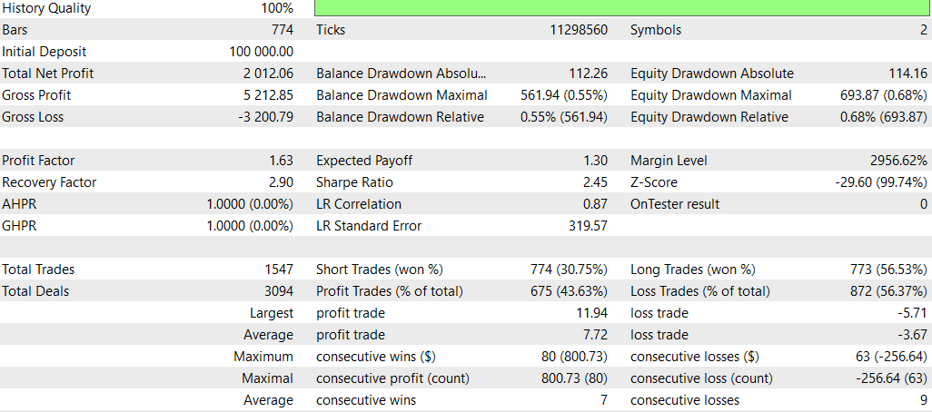
Overall, the non-DL strategy appears to have performed better in terms of total profitability and risk-adjusted returns, despite having a higher maximum draw-down. It traded more actively and seemed more effective with long positions. The DL strategy was more conservative, with lower draw-downs but also lower overall returns.

However, it's important to note that this comparison is based on a single back test period. To draw more robust conclusions, you'd want to test these strategies across multiple time periods and market conditions.

Conclusion

This study explored the integration of Deep Learning (DL) models into three advanced trading Expert Advisors (EAs): Causality Network Analysis (CNA), Stochastic Optimization and Optimal Control (SMOC), and Nash's Game Theory. The process involved creating ONNX models using Python and incorporating them into existing MQL5 scripts.

The results of this integration were mixed across the different strategies:

1. For the CNA strategy, the DL version showed more conservative trading with lower returns but also lower risk compared to the non-DL version. While less profitable, it demonstrated better consistency and a more balanced approach to trading.
2. In the case of SMOC, the DL version outperformed its non-DL counterpart significantly. It showed better profitability, higher win rates, and superior risk-adjusted returns, suggesting that the DL model effectively enhanced the strategy's decision-making process.
3. For Nash's Game Theory approach, the non-DL version performed better overall, with higher total profitability and risk-adjusted returns, despite having a higher maximum draw-down. The DL version traded more conservatively but achieved lower overall returns.

These results highlight the potential of integrating Deep Learning into trading strategies, but also underscore the importance of careful implementation and testing. The effectiveness of DL integration varies depending on the underlying strategy and market conditions.

It's crucial to note that these findings are based on specific back test periods and market conditions. To draw more robust conclusions, further testing across various time frames and market scenarios would be necessary.

In conclusion, while Deep Learning can enhance trading strategies, its integration should be approached cautiously and with thorough testing. The mixed results across different strategies suggest that the effectiveness of DL in trading is not universal and depends heavily on the specific strategy and market context. Future research could explore optimizing these DL models for different time frames and market conditions to potentially improve their performance across various trading scenarios.