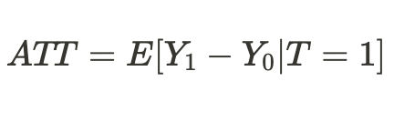
Causal inference in time series classification problems

Article content:

• Introduction
• History of the causal inference
• Causal inference basics in machine learning
• Evidence Ladder in causal inference
• Notation in causal inference
• Bias
• Randomized experiments
• Matching
• Uncertainty
• Meta learners
• An example of building a trading system

In the previous article, we have thoroughly examined training via meta learner and cross-validation, as well as saving models in the ONNX format. I have also noted that machine learning models are not capable of finding patterns out of the box in disparate and contradictory data. In this case, it is very important what exactly is sent to the input and output of a neural network or any other machine learning algorithm.

On the other hand, we cannot always prepare the necessary training data, whose structure already contains causal relationships. As a rule, this is a set of indicators and examples of buy and sell scenarios. The incremental sign, zigzag, or position of moving averages relative to each other is often used to set the direction of a future trade. All these types of markings are not expert and, as a rule, do not contain true causal relationships.

Data tagging is perhaps the most expensive and time- and resource-consuming process in the world of machine learning as it requires the involvement of specialists in the field under study (so-called annotators). Even powerful language neural networks like GPT and their analogues, trained on large amounts of data, are only able to classify language patterns that form a semantic context. However, they do not answer the question of whether any particular statement is actually true or false. Teams of annotators work with these models, adjusting their answers so that they become useful to the end user.

In this case, the trader has a reasonable question: if I know how to label data, then why do I need a neural network? After all, I can simply write logic based on my knowledge and use it effectively. This idea is right and wrong at the same time. It is wrong in that the neural network copes well with the task of prediction, so it is enough to train it on well-labeled data and then receive predictions on new ones, without bothering to write the logic of the trading strategy. Moreover, the built-in functionality allows evaluating the reliability of predictions using new data. And it is right in that without knowing what to feed into the neural network input or by supplying incorrectly labeled data as output, it will not be able to create a profitable trading strategy by default.

Understanding of the above problems of machine learning did not come to traders immediately. Initially, even the creators of the first simple machine learning algorithms firmly believed that the mathematical analogue of a neuron copies the work of brain neurons, which means that a sufficiently large neural network will be able to fully perform the functions of the brain and learn to analyze information independently. Later it was understood that the brain features a large number of highly specialized departments. Each of them processes certain information and transmits it to other departments. This is how multilayer neural network architectures emerged, thanks to which researchers came closer to unraveling the mysteries of how the brain works. Such architectures have learned to perfectly process specific information, such as visual, text, audio or tabular data.

As it turned out later, such neural networks also do not have the ability to make independent conclusions regarding true patterns, while engaged in supervised learning. They are prone to overtraining and subjectivity.

The next step on the path to understanding the structure and functioning of the brain was the discovery that natural neural networks are based on reinforcement learning, and not just on learning from ready-made samples. This is a type of learning, in which a complex system is rewarded for subjectively correct decisions and penalized for incorrect ones. After receiving such rewards multiple times, depending on the task at hand, experience is accumulated and subjectively correct answer options are learned. The brain or neural network begins to make fewer mistakes in certain cases if it has already encountered them before.

This led to the emergence of reinforcement learning, when researchers themselves set the reward function (some kind of fitness function in optimization algorithms), rewarding or punishing the neural network for correct or incorrect answers. Now the machine learning algorithm is no longer trained on ready-made well-labeled data, but acts by trial and error, trying to maximize the reward function. Currently, there are a large number of reinforcement learning algorithms for different tasks, and this area is developing quite actively.

This seemed like a breakthrough until it began to be used, among other things, for problems of classifying financial time series. It became clear that such learning is very difficult to control, since now everything comes down to setting the right reward function and choosing the right network architecture. We face the same trivial problem: if we do not know the true objective function, which describes the real causal relationships between the states of the system and its responses, then we are unlikely to find it through numerous searches of both the objective function itself and various reinforcement learning algorithms unless you are lucky.

Much the same story happened with generative models that learn conditionally without a supervisor. Built on the principle of an encoder-decoder or generator-discriminator, they learn to compress information, highlighting important features, or distinguish real samples from fictitious ones (in the case of adversarial neural networks), and then generate plausible examples, such as images. While everything is more or less clear with images and they are a kind of plausible "nonsense" of a neural network, it is all much more complicated with the generation of accurate consistent answers. The element of randomness inherent in the generation of a particular answer does not allow us to draw unambiguous conclusions about causal relationships, which is not suitable for such a risky activity as trading, where the random behavior of the algorithm is a synonym to losses.

The author of the article tried all these algorithms for time series classification problems, in particular Forex currency pairs, and was not too satisfied with the results.

Recently, we can increasingly come across publications on the topic of so-called "reliable" or "trustworthy" machine learning. In general, the set of approaches is not yet fully formed and varies from area to area. It is important to understand that it addresses the problem of causal inference through machine learning algorithms. Researchers have learned to understand and trust machine learning so much that they are ready to entrust it with the task of searching for causal relationships in data, which, of course, takes machine learning to a completely new level. Causal inference is widely used in fields such as medicine, econometrics and marketing.

This article describes an attempt to understand some causal inference techniques in relation to algorithmic trading.

History of the causal inference

Causality has a long history and has been considered in most, if not all, advanced cultures known to us.

Aristotle, one of the most prolific philosophers of ancient Greece, argued that understanding the causal structure of a process is a necessary component of knowing about that process. Moreover, he argued that the ability to answer "why" questions is the essence of scientific explanation. Aristotle identifies four types of causes (material, formal, efficient and final). This idea may reflect some interesting aspects of reality, although it may sound counterintuitive to a modern person.

David Hume, the famous 18th-century Scottish philosopher, proposed a more unified framework for causal relationships. Hume began by arguing that we never observe causal relationships in the world. The only thing we observe is that some events are connected with each other: We only find that one of them actually follows the other. The momentum of one billiard ball is accompanied by the movement of the second. This is the whole that appears to the external senses. The mind experiences no feelings or internal impressions from this succession of objects: there is therefore nothing in each particular phenomenon to suggest any force or necessary connection.

One interpretation of Hume's theory of causation is as follows:

1. We only observe how the movement or appearance of object A precedes the movement or appearance of object B.
2. If we see this sequence enough times, we develop a sense of anticipation.
3. This feeling of expectation is the essence of our concept of causality (it is not about the world, it is about the feeling that we develop)

This theory is very interesting from at least two points of view. First, elements of this theory are very similar to an idea called conditioning in psychology. Conditioning is a form of learning. There are many types of conditioning, but they all rely on a common basis - association (hence the name of this type of learning - associative learning). In any type of conditioning, we take some event or object (usually called a stimulus) and associate it with a specific behavior or response. Associative learning works in different animal species. It can be found in humans, monkeys, dogs and cats, as well as in much simpler organisms such as snails.

Secondly, most classical machine learning algorithms also work based on associations. In case of supervised learning, we try to find a function that maps inputs to outputs. To do this efficiently, we need to figure out which elements of the input are useful for predicting the output. In most cases, association is enough for this purpose.

Additional information about the possibilities of studying causal relationships comes from child psychology.

Alison Gopnik is an American child psychologist who studies how infants develop models of the world. She also collaborates with computer scientists to help them understand how human infants construct common sense concepts about the external world. Children use associative learning even more than adults, but they are also insatiable experimenters. Have you ever seen a parent trying to convince their child to stop throwing toys around? Some parents tend to interpret this behavior as rude, destructive or aggressive, but kids often have other motives. They conduct systematic experiments that allow them to study the laws of physics and the rules of social interaction (Gopnik, 2009). Infants as young as 11 months prefer to experiment with objects that exhibit unpredictable properties rather than with objects that behave predictably (Stahl & Feigenson, 2015). This preference allows them to effectively build models of the world.

What we can learn from babies is that we are not limited to observing the world, as Hume assumed. We can also interact with it. In the context of causal inference, these interactions are called interventions. Interventions are at the heart of what many consider the Holy Grail of the scientific method: the randomized controlled trial (RCT).

But how can we distinguish an association from a real causal relationship? Let's try to figure it out.

Causal inference basics in machine learning

The main goal of causal inference in machine learning is to determine whether we can make decisions based on a trained machine learning algorithm. Here we are not always interested in the accuracy and frequency of predictions, although this is also important, but we are more interested in their stability and our level of confidence in them.

The main thesis of causal inference is: "Correlation does not imply causation". This means that correlation does not prove the influence of one event on another, but only determines the linear relationship of these two or more events.

Therefore, a causal relationship is determined through the influence of one variable on another. The influencing variable is often called instrumental in the case of third-party intervention, or simply one of the covariates (features in machine learning). Or through some action to another action. In general, is event A always followed by event B? Or does event A actually cause event B? This is why it is also called A/B testing. This is exactly what we will deal with further, but using machine learning algorithms.

There are a number of approaches to tackle the inference of causality, both using randomized experiments and using instrumental variables and machine learning. It makes no sense to list all the methods here, since other works are devoted to this. We are interested in how we can apply this to a time series classification problem.

It is important to note that almost all of these methods are based on Neumann-Rubin causal model, or models of potential results (outcomes). This is a statistical approach that helps determine whether one event is actually a consequence of another.

For example, a trained classifier shows profits on the training and validation subsamples, while its signals lead to losses on the test subsample. To measure the causal effect on new data using this classifier, we need to compare the results on new data in case it was actually trained and in case it was not trained. Since it is impossible to see the results of an untrained classifier because it does not generate any buy or sell signals, this potential outcome is unknown. We only have the actual result after training it, and the unknown result without training is counterfactual. In other words, we need to find out whether training a classifier leads to increased profits or to making a profit on new data compared to, say, opening trades at random. That is, does training a classifier have any positive effect at all?

This dilemma is a "fundamental problem of causal inference", when we do not know what the actual result would have been if the classifier had not been trained, but we only know the actual result after it has been trained.

Due to the fundamental problem of causal inference, causal effects at the unit level (a single training example) cannot be directly observed. We cannot say with certainty whether our predictions have improved because we have nothing to compare it to. However, randomized experiments allow us to evaluate causal effects on population level. In a randomized experiment, classifiers are randomly trained on different subsamples. Because of this random distribution of training examples, the classifiers' prediction results are (on average) equivalent, and the difference in classifier predictions for specific examples can be attributed to the case of examples from the test set being included or not being included in the training examples. We can then obtain an estimate of the average causal effect (also called the average treatment effect) by calculating the difference in the average results between the treated (with a trained classifier on the data) and control (with an untrained classifier on the data) samples.

Or imagine that there is a multiverse and in each of the subuniverses the same person lives, who makes different decisions that lead to different results (outcomes). The person in each subuniverse knows only his or her own version of the future and does not know the options for the future of his or her other "selves" in other subuniverses.

In the multiverse example, we assume that all people have counterparts in other universes. All people are, on average, similar. This means that we can compare the reasons for the decisions they make with the results of those decisions. Thus, based on this knowledge, it will be possible to draw a causal conclusion about what would happen to a specific person in another universe if he or she acted in one way or another that he or she had never acted there before. If, of course, these universes are similar.

Evidence Ladder in causal inference

There is some systematization of causal inference methods, which represents a hierarchy of methods according to their evidentiary ability. This will help to find out what evidentiary power our chosen method will have. Below are citations from the article, the link to which is provided above.

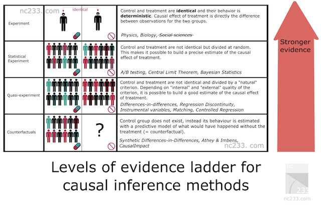
• On the first rung of the ladder sit typical scientific experiments.

The kind you were probably taught in middle or even elementary school. To explain how a scientific experiment should be conducted, my biology teacher had us take seeds from a box, divide them into two groups and plant them in two jars. The teacher insisted that we made the conditions in the two jars completely identical: same number of seeds, same moistening of the ground, etc. The goal was to measure the effect of light on plant growth, so we put one of our jars near a window and locked the other one in a closet. Two weeks later, all our jars close to the window had nice little buds, while the ones we left in the closet barely had grown at all. The exposure to light being the only difference between the two jars, the teacher explained, we were allowed to conclude that light deprivation caused plants to not grow.

This is basically the most rigorous you can be when you want to attribute cause. The bad news is that this methodology only applies when you have a certain level of control on both your treatment group (the one who receives light) and your control group (the one in the cupboard). Enough control at least that all conditions are strictly identical but the one parameter you’re experimenting with (light in this case). Obviously, this doesn’t apply in social sciences nor in data science.

Then why does the author include it in the article you might ask? Well, basically because this is the reference method. All causal inference methods are in a way hacks designed to reproduce this simple methodology in conditions where you shouldn’t be able to make conclusions if you followed strictly the rules explained by your middle school teacher.

• Statistical Experiments (aka A/B tests)

Probably the most well-known causal inference method in tech: A/B tests, a.k.a Randomized Controlled Trials. The idea behind statistical experiments is to rely on randomness and sample size to mitigate the inability to put your treatment and control groups in the exact same conditions. Fundamental statistical theorems like the law of large numbers, the Central Limit theorem or Bayesian inference gives guarantees that this will work and a way to deduce estimates and their precision from the data you collect.

• Quasi-Experiments

A quasi-experiment is the situation when your treatment and control group are divided by a natural process that is not truly random but can be considered close enough to compute estimates. In practice, this means that you will have different methods that will correspond to different assumptions about how “close” you are to the A/B test situation. Among famous examples of natural experiments: using the Vietnam war draft lottery to estimate the impact of being a veteran on your earnings, or the border between New Jersey and Pennsylvania to study the effect of minimum wages on the economy.

• Counterfactual methods

Here we abandon the idea of treatment and control groups (actually, not entirely), and, in fact, model the time series Y from historical data without the participation of X in the future, where X already comes into play. Thus, during the experiment, we can compare the actual data of Y (where X participated) with the model (prediction of Y without X) and guess the effect size, adjusting it for the accuracy of the model for Y. However, for this assumption to be close to the truth, we need to do the greatest number of tests for the stability of the method. The resulting effect will critically depend not only on the quality of the model, but also, in general, on the correct application of the chosen method.

When building a time series classification model, we can only use counterfactual methods. In other words, we need to come up with an instrumental variable or treatment ourselves, apply it to our observations, and then conduct appropriate tests for the method stability, which is what we will do in the future. Obviously, this is the most complex approach and it has the least evidentiary strength according to the Evidence Ladder.

Notation in causal inference

We agreed that "treatment" T refers to some impact on an object, be it a clinic patient, a person under the influence of an advertising campaign, or some sample from the training set. Then there are two options. Either the subject received treatment or not.

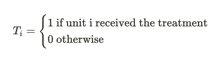
We also already know that each object (unit) cannot be treated and not treated at the same time. That is, it could be one of two things.

So,

indicate the potential outcomes for a unit without treatment and for a unit with treatment. We can calculate the individual treatment effect through the difference of these potential outcomes:

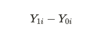
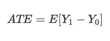
Due to the fundamental problem of causal inference noted above, we cannot obtain an individual treatment effect because only one of the outcomes is known, but we can calculate the average treatment effect across all similar subjects, some of which received the treatment while some did not:

Or we can get an average treatment effect only for units that have been treated:

Bias

Bias is what distinguishes correlation (association) from causation (cause and effect). What if, in another universe, our "selves" found themselves in completely different conditions of existence, and the results of the decisions they made would no longer correspond to those we are accustomed to in this universe. Then conclusions about possible outcomes will turn out to be erroneous, and assumptions will only be associative, but not causal relationships.

This is also true for trained classifiers when they stop making profit on new data they have not seen before or they simply stop predicting correctly.

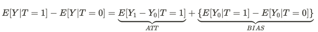
This equation answers the question why an associative relationship is not a causal one. Bias here is how different the living conditions of people in different universes are before they have any effect in both universes. This is because there are many other variables that influence the outcome of the decision they make. As a result, the populations of people in one universe and in another differ not only in that different decisions are made, but also in different conditions of existence.

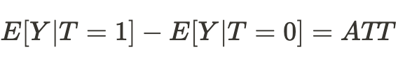
It turns out that if the conditions of our existence in different universes turned out to be comparable, then our conclusion regarding the results of our actions (on average) in another universe will turn out to be causal:

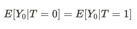
Accordingly, the difference of means now becomes the average causal effect:

We can simply conclude that to estimate a causal effect, a sample from one universe should be comparable to a sample from another universe. If this is so, then we will be able to determine the true relationship and with a high degree of probability we will be able to predict the result of actions of our "selves" in another universe.

In other words, an association becomes a causal relationship when bias is equal to zero.

Translating the above into machine learning terms, we usually deal with training and validation data, as well as test data. The machine training model learns using training data with partial participation of validation data. If the subsamples are comparable, then we will have approximately the same prediction errors on the training and validation data. If the subsamples differ by a conditional bias, then the prediction error on the validation data will be larger. Not to mention the test subsample, the data distribution of which may not be at all similar to the distributions of the first two.

But how can we then make a causal inference if the distributions of the subsamples are different? The answer has partially been given in the previous section already: we can make causal inferences through randomized experiment.

Randomized experiments

As has already become clear, randomization allows us to randomly divide data into groups, one of which received "treatment" (in our case, model training), while the other did not. Moreover, we should do this several times and train many models. This is necessary in order to eliminate bias from our estimates. Randomizing and training multiple classifiers removes the dependence of potential outcomes on one specific machine learning model.

This may be a little confusing at first. We might think that the lack of dependence of outcomes (predictions) on a particular model makes training that model useless. From the point of view of the predictions of this particular model, the answer is yes. However, we are dealing with potential outcomes (predictions).

Potential outcome is what the outcome would be if the model were trained or not trained. In randomized experiments, we do not want the outcome (prediction) to be independent of training, since model training directly affects the outcome.

But we want potential outcomes to be independent of training any particular classifier, which is biased!

By saying this, we mean that we want the potential outcomes to be the same for the control and test groups. Our training and test data need to be comparable because we want to remove bias from the estimates. But each individual classifier gives different weights to different training examples, even if they are mixed, which makes the amount of treatment different for each observation. This complicates causal inference.

Randomization of training examples allows us to evaluate the effect of treatment (training) by obtaining the difference in model errors on the test and training samples. However, in the case of classification, the features of machine learning algorithms should be taken into account. In this case, the effect estimate is still biased because each individual classifier is trained on half or more of the original examples, giving each example different weights (treatment). By using multiple classifiers (an ensemble of them), we minimize bias by averaging the classifier scores, making the treatment more equal for each unit. This puts all training examples in the same conditions, giving them the same value.

In this section, we learned that randomized experiments help remove bias from the data to make more reliable causal inferences. Model ensembles help us give equivalent estimates of training effect.

Matching

Randomized experiments allow us to estimate the average effect of training an ensemble of models. However, we are interested in obtaining individual effects for each training example. This is necessary in order to understand in what situations the trading strategy, on average, brings profit, and what situations should be adjusted or excluded from trading. In other words, we want to obtain conditional estimates of the effects of training, depending on the individual characteristics of each object.

Matching is a way to compare individual samples from the entire sample to make sure that they are similar in all other characteristics except whether they were included in the training set or not. This allows us to derive individual scores for each training example.

There is exact and imprecise (approximate) matching.

In rough matching, for example, we can compare all units based on proximity criteria such as Euclidean distance, as well as Minkowski and Mahalanobis distances. But since we are dealing with time series, we have the option to compare units positionally, by time. If we train an ensemble of models, then the predictions of each model at any given time are already associated with the set of features present at that point on the timeline. All we have to do is compare the predictions of all models for a specific time point. The computational complexity of such a comparison is minimal compared to other methods, which will allow for more experiments. In addition, this will be an accurate matching.

Uncertainty

In algorithmic trading, it is not sufficient for us to determine the average and individual treatment effects, because we want to build the final classifier model. We need to apply causal inference tools to estimate the uncertainty in the dataset and divide units into those that respond to conditional treatment (training a classifier) and those that do not. In other words, into those that, in the vast majority of cases, are classified correctly and incorrectly. Depending on the degree of uncertainty, which is calculated as the sum of the differences between the potential outcomes for all ensemble models.

Since we are estimating the uncertainty of the data from the classifier point of view, buy and sell orders should be evaluated separately because their joint distribution will confound the final estimate.

Meta learners

Meta learners in causal inference are machine learning models that help estimate causal effects.

We have already become familiar with ATE and ATT concepts, which give us information about the average causal effect in a population. However, it is important to remember that people and other complex organisms (for example, animals, social groups, companies or countries) can respond differently to the same treatment. When we deal with a situation like this, ATE can hide important information from us. 

One solution to this problem is to calculate CATE (conditional average treatment effect), also known as HTE. When calculating CATE, we look not just at the treatment, but at a set of variables that define the individual characteristics of each unit that can change how the treatment affects the outcome.

In the case of binary treatment, CATE can be defined as:

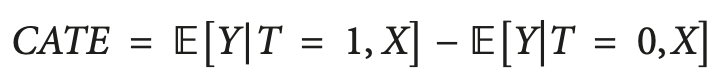
where X are the characteristics that describe each individual object (unit). Thus, we make a transition from a homogeneous treatment effect to a heterogeneous one.

The idea that people or other units can react differently to the same treatment is often represented in the form of a matrix, sometimes called an uplift matrix, which you can see in the figure.

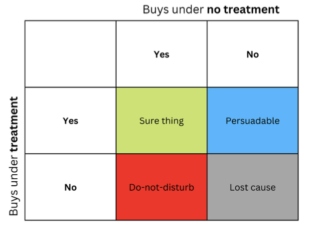
The strings represent the response to the content when the message (such as an advertisement) is presented to the recipient. Columns represent responses when no treatment is given.

The four colored cells represent the dynamics of the treatment effect. Confident buyers (green) buy regardless of treatment. Reds (Do Not Disturb) can buy without treatment, but will not buy if treated. Those who have lost interest (gray) will not buy regardless of treatment status, and blue ones will not buy without treatment, but may buy if approached.

If you are a marketer on a budget, you want to focus on marketing to the blue group (Persuadable) and avoid marketing to the red group (Do Not Disturb) if possible.

Marketing in the "Sure thing" and "Lost cause" groups will not cause you direct harm, but it will not provide any benefit either.

Likewise, if you are a doctor, you want to prescribe a medicine to people who might benefit from it and avoid prescribing it to those who might be harmed by it. In many real-world scenarios, the outcome variable can be probabilistic (for example, the probability of a purchase) or continuous (for example, the amount of spending). In such cases, we are unable to identify discrete groups and focus on finding the units with the largest expected increase in the outcome variable between the no-treatment and treatment conditions. This difference between outcome with treatment versus no treatment is sometimes called an uplift.

Translating this into the language of time series classification, we need to determine which examples from the training set respond best to treatment (classifier training) and put them in a separate group.

One simple way to estimate a heterogeneous treatment effect is to build a surrogate model that predicts the treatment variable based on the predictors you use, formally represented as follows: 

T ~ X

The performance of such a model should be essentially random. If it is non-random, it would mean that treatment depends on the traits, which means there is some missing variable that we did not take into account, and it affects our causal inferences, introducing confusion. This often happens due to poor randomized controlled trial design, where the treatment is not actually randomly assigned.

S-Learner

S-Learner is the name of a simple approach to CATE modeling. S-Learner belongs to the category of so-called meta learners. Note that causal meta learners are not directly related to the concept of meta learning used in traditional machine learning. They take one or more basic (traditional) machine learning models and use them to calculate the causal effect. In general, you can use any machine learning model of sufficient complexity (tree, neural network, etc.) as a base learner if it is compatible with your data.

S-Learner is the simplest meta model that uses only one basic learner (hence its name: S(ingle)-Learner). The idea behind S-Learner is surprisingly simple: train one model on the full training data set, including the treatment variable as a feature, predict both potential outcomes and subtract the results to get CATE.

After training, the step-by-step forecasting procedure for S-Learner is as follows:

1. Select the observation of interest.
2. Set the treatment value for this observation to 1 (or True).
3. Predict the outcome using the trained model.
4. Take the same observation again.
5. This time set the treatment value to 0 (or False).
6. Make a prediction.
7. Subtract the prediction value without treatment from the prediction value with treatment.

T-Learner

The main motivation of T-Learner is to overcome the main limitation of S-Learner. If S-Learner can learn to ignore treatment, then why not make it impossible to ignore it?

That is exactly what T-Learner is. Instead of fitting one model to all observations (treated and untreated), we now fit two models — one only for the treated units and one only for the untreated units.

In some ways, this is equivalent to forcing the first split in a tree-based model to be a split by the treatment variable.

The T-Learner learning process is as follows:

1. Divide the data by the treatment variable into two subsets.
2. Train two models - one on each subset.
3. For each observation, predict the results using both models.
4. Subtract the results of the model without treatment from the results of the model with treatment.

Note that there is now no chance that treatments will be ignored because we have coded the treatment split as two separate models.

T-Learner focuses on improving just one aspect where S-Learner can (but does not have to) fail. This improvement comes at a cost. Fitting two algorithms to two different subsets of data means that each algorithm is trained on less data, which can reduce the quality of the fit.

This also makes T-Learner less efficient in terms of data usage (we need twice as much data to train each T-Learner base learner to produce a representation comparable in quality to S-Learner). This typically results in greater variance in the T-Learner score compared to the S-Learner one. In particular, variance can become very large in cases where one treatment group has far fewer observations than the other.

To summarize, T-Learner can be useful when you expect the treatment effect to be small and S-Learner may not recognize it. One thing to keep in mind is that this meta learner is generally more data-intensive than S-Learner, but the difference decreases as the overall size of the dataset increases.

X-Learner

X-Learner is a meta learner designed to make more efficient use of the information available in data. 

X-Learner seeks to estimate CATE directly and, in doing so, uses information that S-Learner and T-Learner previously discarded. What kind of data is this? S-Learner and T-Learner studied what is called the response function, or how units respond to treatment (in other words, the response function is the mapping of trait X and treatment T to outcome y). At the same time, none of the models used the real result to simulate CATE. 

1. The first step is simple, and you already know it. That is exactly what we did with T-Learner. We split our data by treatment variable so as to obtain two separate subsets: the first containing only the units that received the treatment, and the second containing only the units that did not receive the treatment. Next, we train two models: one on each subset. 
2. We introduce an additional model called the "propensity score model" (in the simplest case it is logistic regression) and train it to predict treatment for X traits.
3. Next, we calculate the treatment effect and train two models on the features and CATE values.
4. The results of using the two models are added with the weight obtained from the propensity score of the model.

With the ability to weight two submodels, X-Learner can be really effective when the data set is highly imbalanced. 

On the other hand, if your dataset is very small, X-Learner may not be the best choice because each additional model comes with additional noise when fitting, and we may not have enough data to use that model. In this case, S-Learner is better suited.

There are more advanced meta learners. I am not going to use them, so there is little point in discussing them in this short article. These are Debiased/orthogonal machine learning and R-learner, which you can study on your own.

Conclusion on existing meta learners

The proposed algorithms, despite a rather extensive theoretical part, are only estimators of the CATE effect. The literature on causal inference hardly touches on the full cycle of detection and evaluation of treatment effects, unless these are some very obvious cases, and the situation with the implementation of the resulting models in business processes is also rather weak. It is stated that it is up to the researcher to formulate the experiments and then use these estimators. I decided to go a little further and incorporated elements of these estimators into creating a trading system, which occurs automatically. Signs and labels are supplied to the input and output of the algorithm, as before, then the algorithm tries to identify causal relationships on the part of the data where this is possible, and exclude the rest from the logic of making trading decisions.

 

Implementation of the meta learner function for building a trading algorithm

Armed with the necessary minimum of knowledge, I propose to consider my own algorithm. Many experiments have been conducted with different meta learners and ways of using them to analyze causal effects. At the moment, the proposed algorithm is one of the best in the arsenal, although it can be improved.

Since we have determined that it is not practical to use a single classifier, which is biased, to evaluate potential outcomes, the first argument of the function is a specified number of classifiers. I used the CatBoost algorithm. Next are the learner hyperparameters, such as the number of iterations and tree depth, as well as bad_samples_fraction - a parameter known from the very first article dedicated to meta learners. This is the percentage of poorly classified examples that should be excluded from the final training set. We should try not to trade at these moments.

BAD_BUY and BAD_SELL are collections of bad example indexes that are replenished at each iteration. 

At each new iteration, the number of which is equal to the specified number of learners, the dataset is divided into training and validation subsamples randomly in a given proportion (here it is 50/50). This keeps each individual algorithm from overtraining. Random partitioning allows each classifier to be trained and validated on unique subsamples, while the entire dataset is used to produce estimates. This eliminates bias in the estimates, allowing us to more accurately assess which examples are actually poorly susceptible to treatment (classifier training).

After each training, the actual class labels are compared with the predicted ones. The incorrectly predicted labels join the collections of bad examples. We hope that as the number of classifiers increases, the estimates of really bad samples become less biased.

After the collections of bad examples are formed, we calculate the average number of bad samples across all indexes. After this, we select those indices in which the number of bad examples exceeds the average by a certain amount. This allows us to vary the number of bad examples included in the training of the final model, since with a large number of retrainings there is a probability that each index will fall into bad examples at least once. In this case, it turns out that all examples will be excluded from the final training set, then this algorithm will not work. 

def meta_learners(models_number: int, iterations: int, depth: int, bad_samples_fraction: float):
    dataset = get_labels(get_prices())
    data = dataset[(dataset.index < FORWARD) & (dataset.index > BACKWARD)].copy()

    X = data[data.columns[1:-2]]
    y = data['labels']

    BAD_BUY = pd.DatetimeIndex([])
    BAD_SELL = pd.DatetimeIndex([])

    for i in range(models_number):
        X_train, X_val, y_train, y_val = train_test_split(
            X, y, train_size = 0.5, test_size = 0.5, shuffle = True)
        
        # learn debias model with train and validation subsets
        meta_m = CatBoostClassifier(iterations = iterations,
                                depth = depth,
                                custom_loss = ['Accuracy'],
                                eval_metric = 'Accuracy',
                                verbose = False,
                                use_best_model = True)
        
        meta_m.fit(X_train, y_train, eval_set = (X_val, y_val), plot = False)
        
        coreset = X.copy()
        coreset['labels'] = y
        coreset['labels_pred'] = meta_m.predict_proba(X)[:, 1]
        coreset['labels_pred'] = coreset['labels_pred'].apply(lambda x: 0 if x < 0.5 else 1)
        
        # add bad samples of this iteration (bad labels indices)
        coreset_b = coreset[coreset['labels']==0]
        coreset_s = coreset[coreset['labels']==1]

        diff_negatives_b = coreset_b['labels'] != coreset_b['labels_pred']
        diff_negatives_s = coreset_s['labels'] != coreset_s['labels_pred']
        BAD_BUY = BAD_BUY.append(diff_negatives_b[diff_negatives_b == True].index)
        BAD_SELL = BAD_SELL.append(diff_negatives_s[diff_negatives_s == True].index)

    to_mark_b = BAD_BUY.value_counts()
    to_mark_s = BAD_SELL.value_counts()
    marked_idx_b = to_mark_b[to_mark_b > to_mark_b.mean() * bad_samples_fraction].index
    marked_idx_s = to_mark_s[to_mark_s > to_mark_s.mean() * bad_samples_fraction].index
    data.loc[data.index.isin(marked_idx_b), 'meta_labels'] = 0.0
    data.loc[data.index.isin(marked_idx_s), 'meta_labels'] = 0.0

    return data[data.columns[1:]]

The remaining functions have not been changed and are described in the previous article. You can download them there, while the meta learner function can be replaced with the proposed one. In the rest of this article, we will focus on the experiments and try to draw final conclusions.

Testing the causal inference algorithm

Let's assume that we use genetic optimization of trading strategies according to some criterion (the so-called fitness function). We are interested not only in the best optimization result, but also in ensuring that the results of all passes, on average, are good. If the trading strategy is bad or the spread of parameters is too large, then there will be a large number of optimization passes with unsatisfactory results, which will negatively affect the average estimate. We would like to avoid this, so we will train our algorithm many times, then average the results and compare the best result with the average.

To do this, I wrote a modification of a custom tester that tests all trained models from the list at once:

def test_all_models(result: list):
    pr_tst = get_prices()
    X = pr_tst[pr_tst.columns[1:]]
    pr_tst['labels'] = 0.5
    pr_tst['meta_labels'] = 0.5
    

    for i in range(len(result)):
        pr_tst['labels'] += result[i][1].predict_proba(X)[:,1]
        pr_tst['meta_labels'] += result[i][2].predict_proba(X)[:,1]

    pr_tst['labels'] = pr_tst['labels'] / (len(result)+1)
    pr_tst['meta_labels'] = pr_tst['meta_labels'] / (len(result)+1)
    pr_tst['labels'] = pr_tst['labels'].apply(lambda x: 0.0 if x < 0.5 else 1.0)
    pr_tst['meta_labels'] = pr_tst['meta_labels'].apply(lambda x: 0.0 if x < 0.5 else 1.0)

    return tester(pr_tst, plot=plt)

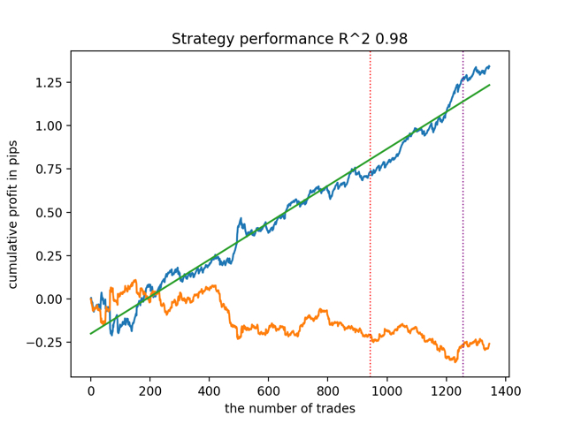
Now we will do causal inference 25 times (we will train 25 independent models, which are highly randomized in terms of random division into subsamples):

options = []
for i in range(25):
    print('Learn ' + str(i) + ' model')
    options.append(learn_final_models(meta_learners(15, 25, 2, 0.3)))

options.sort(key=lambda x: x[0])
test_model(options[-1][1:], plt=True)
test_all_models(options)

Let's first test the best model according to R^2 version:

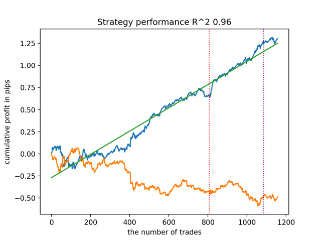
Then test all the models at once:

The average result is not much different from the best. This means that in the course of a controlled randomized experiment it is possible to get closer to true causal relationships.

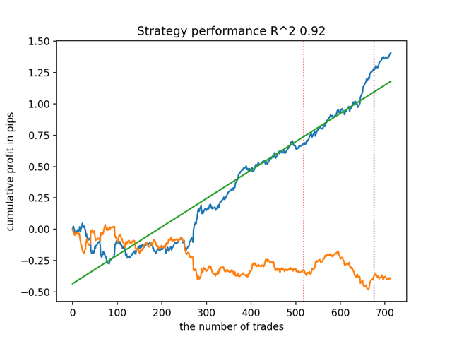
Let's train and test the algorithm with other meta learner input parameters.

options = []
for i in range(25):
    print('Learn ' + str(i) + ' model')
    options.append(learn_final_models(meta_learners(5, 10, 1, 0.4)))

options.sort(key=lambda x: x[0])
test_model(options[-1][1:], plt=True)
test_all_models(options)

The results are as follows:

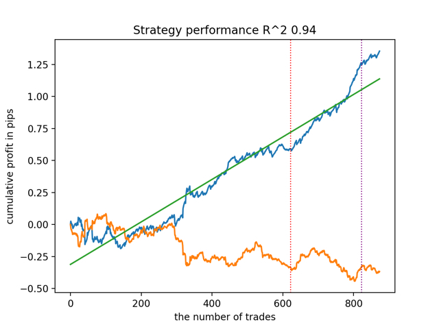
It was also noted that the depth of the training history (highlighted by vertical lines in the graphs) affects the quality of the results, as well as the number of features and other hyper parameters of the models (which is generally not surprising), while the spread in the quality of the models remains small. I believe that the resulting stability is an important property or feature of the proposed algorithm, which allows us to have additional confidence in the quality of the resulting trading strategies.

Summary

This article introduced you to the basic concepts of causal inference. This is a fairly broad and complex topic to cover all its aspects in one article. Causal inference and causal thinking have their roots in philosophy and psychology and play an important role in our understanding of reality. Therefore, much of what is written is well perceived on an intuitive level. However, being somewhat agnostic, I tried to give a practical, illustrative example to demonstrate the power of so-called causal inference in time series classification problems. You can use this algorithm to conduct various experiments. Just replace a couple of functions in the code presented in the previous article. The experiments do not end there. Perhaps, new interesting information will appear, which I will later share with you.

Useful references

• Aleksander Molak "Causal inference and discovery in Python"
• Matheus Facure "Causal inference for the Brave and True"
• Miguel A. Hernan, James M. Robins "Causal inference: What If"
• Gabriel Okasa "Meta-learners for estimation of causal effects: finite sample cross-fit performance"