
Application of Nash's Game Theory with HMM Filtering in Trading
Introduction
Applying mathematical theories can provide a strategic advantage. One such theory is the Nash Equilibrium, developed by the renowned mathematician John Forbes Nash Jr. Known for his contributions to game theory, Nash's work has been influential across various fields, including economics and beyond. This article explores how Nash's equilibrium theory can be effectively applied to trading. By utilizing Python scripts and advanced statistical models, we aim to harness the principles of Nash's game theory to optimize trading strategies and make more informed decisions in the market.Nash

Who is John Forbes Nash Jr.?
Wikipedia says of him:
John Forbes Nash, Jr. (June 13, 1928 – May 23, 2015), known and published as John Nash, was an American mathematician who made fundamental contributions to game theory, real algebraic geometry, differential geometry, and partial differential equations. Nash and fellow game theorists John Harsanyi and Reinhard Selten were awarded the 1994 Nobel Prize in Economics. In 2015, he and Louis Nirenberg were awarded the Abel Prize for their contributions to the field of partial differential equations.
As a graduate student in the Princeton University Department of Mathematics, Nash introduced a number of concepts (including Nash equilibrium and the Nash bargaining solution) which are now considered central to game theory and its applications in various sciences.
There is a film based on his life entitled "A Beautiful Mind". We are going to apply his game theory to trading with MQL5.
How are we going to introduce Nash's Game Theory in trading?
Nash Equilibrium Theory
Nash Equilibrium is a concept in game theory where each player is assumed to know the equilibrium strategies of the other players, and no player has anything to gain by changing only their own strategy.
In a Nash equilibrium, each player's strategy is optimal given the strategies of all other players. A game may have multiple Nash equilibria or none at all.
The Nash equilibrium is a fundamental concept in game theory, named after mathematician John Nash. It describes a state in a non-cooperative game where each player has chosen a strategy, and no player can benefit by unilaterally changing their strategy while the other players keep theirs unchanged.
Formal definition:
Let (N, S, u) be a game with:
- N players: N = {1, 2, ..., n}
- Strategy sets for each player: S = (S₁, S₂, ..., Sₙ)
- Utility functions for each player: u = (u₁, u₂, ..., uₙ)
A strategy profile s* = (s₁*, s₂*, ..., sₙ*) is a Nash equilibrium if, for each player i and for all alternative strategies sᵢ ∈ Sᵢ:
uᵢ(s₁*, ..., sᵢ*, ..., sₙ*) ≥ uᵢ(s₁*, ..., sᵢ, ..., sₙ*)
In other words, no player i can unilaterally improve their utility by deviating from their equilibrium strategy sᵢ* to any other strategy sᵢ, given that all other players maintain their equilibrium strategies.
For a two-player game, we can express this more concisely:
(s₁*, s₂*) is a Nash equilibrium if:
- u₁(s₁*, s₂*) ≥ u₁(s₁, s₂*) for all s₁ ∈ S₁
- u₂(s₁*, s₂*) ≥ u₂(s₁*, s₂) for all s₂ ∈ S₂
This formulation emphasizes that each player's strategy is a best response to the other player's strategy in equilibrium.
It's important to note that:
- Not all games have a Nash equilibrium in pure strategies.
- Some games may have multiple Nash equilibria.
- A Nash equilibrium is not necessarily Pareto optimal or the most desirable outcome for all players collectively.
The concept of Nash equilibrium has wide-ranging applications in economics, political science, and other fields where strategic interactions between rational agents are studied.
Although in a Nash equilibrium no one can unilaterally improve their position without others adapting, in practice, financial markets are dynamic and rarely in perfect equilibrium. Opportunities to make money arise from temporary inefficiencies, informational advantages, better risk management, and the ability to react more quickly than other players. In addition, external and unpredictable factors can upset the balance, creating new opportunities for those who are prepared.
Fist of all, we have to select the currencies (we are going to do Nash's equilibrium, so we need two symbols, we will choose negatively correlated symbols), we will use python for this. This is the script used:
import MetaTrader5 as mt5
import pandas as pd
from scipy.stats import pearsonr
from statsmodels.tsa.stattools import coint
import numpy as np
import datetime

# Connect with MetaTrader 5
if not mt5.initialize():
    print("Failed to initialize MT5")
    mt5.shutdown()

# Get the list of symbols
symbols = mt5.symbols_get()
symbols = [s.name for s in symbols if s.name.startswith('EUR') or s.name.startswith('USD') or s.name.endswith('USD')]  # Filter symbols by example

# Download historical data and save in dictionary
data = {}
for symbol in symbols:
    start_date = "2020-01-01"
    end_date = "2023-12-31"
    timeframe = mt5.TIMEFRAME_H4
    start_date = datetime.datetime.strptime(start_date, "%Y-%m-%d")
    end_date = datetime.datetime.strptime(end_date, "%Y-%m-%d")
    rates = mt5.copy_rates_range(symbol, timeframe, start_date, end_date)

    if rates is not None:
        df = pd.DataFrame(rates)
        df['time'] = pd.to_datetime(df['time'], unit='s')
        data[symbol] = df.set_index('time')['close']

# Close connection with MT5
mt5.shutdown()

# Calculate the Pearson coefficient and test for cointegration for each pair of symbols
cointegrated_pairs = []
for i in range(len(symbols)):
    for j in range(i + 1, len(symbols)):
        if symbols[i] in data and symbols[j] in data:
            common_index = data[symbols[i]].index.intersection(data[symbols[j]].index)
            if len(common_index) > 30:  # Ensure there are enough data points
                corr, _ = pearsonr(data[symbols[i]][common_index], data[symbols[j]][common_index])
                if abs(corr) > 0.8:  # Strong correlation
                    score, p_value, _ = coint(data[symbols[i]][common_index], data[symbols[j]][common_index])
                    if p_value < 0.05:  # P-value less than 0.05
                        cointegrated_pairs.append((symbols[i], symbols[j], corr, p_value))

# Filter and show only cointegrated pairs with p-value less than 0.05
print(f'Total pairs with strong correlation and cointegration: {len(cointegrated_pairs)}')
for sym1, sym2, corr, p_val in cointegrated_pairs:
    print(f'{sym1} - {sym2}: Correlation={corr:.4f}, P-Cointegration value={p_val:.4f}')
This script firstly initialize MetaTrader 5, then it gets all the symbols starting with EUR or USD or ending in USD. After this it downloads the data from those symbols and shuts down MetaTrader 5. It compares all the symbols and passes only the strong correlated ones and then makes another filter for the strongly cointegrated pairs. It finishes by showing in the terminal the symbols that are left.
Correlation measures how two things are related. Imagine you and your best friend always go to the movies together on Saturdays. This is an example of correlation: when you go to the cinema, your friend is also there. If the correlation is positive, it means when one increases, the other does too. If negative, one increases while the other decreases. If the correlation is zero, it means there is no connection between the two.
Cointegration is a statistical concept used to describe a situation where two or more variables have some long-term relationship, even though they may fluctuate independently in the short term. Imagine two swimmers tied together with a rope: they can swim freely in the pool, but they can't move far from each other. Cointegration indicates that despite temporary differences, these variables will always return to a common long-term equilibrium or trend.
Pearson Coefficient measures how linearly related two variables are. If the coefficient is close to +1, it indicates a direct dependence as one variable increases, so does the other. A coefficient close to -1 means that as one increases, the other decreases, indicating an inverse relationship. A value of 0 means no linear connection. For example, measuring the temperature and the number of cold drink sales can help understand how these factors are related using the Pearson Coefficient.
The results are of the script should look like this ones (this where the results obtained for the scripts initial conditions):
    start_date = "2020-01-01"
    end_date = "2023-12-31"
    timeframe = mt5.TIMEFRAME_H4
Total pairs with strong correlation and cointegration: 40
USDJPY - EURCHF: Correlation=-0.9416, P-Cointegration value=0.0165
USDJPY - EURN.NASDAQ: Correlation=0.9153, P-Cointegration value=0.0008
USDCNH - USDZAR: Correlation=0.8474, P-Cointegration value=0.0193
USDRUB - USDRUR: Correlation=0.9993, P-Cointegration value=0.0000
AUDUSD - USDCLP: Correlation=-0.9012, P-Cointegration value=0.0280
AUDUSD - USDILS: Correlation=-0.8686, P-Cointegration value=0.0026
NZDUSD - USDNOK: Correlation=-0.9353, P-Cointegration value=0.0469
NZDUSD - USDILS: Correlation=-0.8514, P-Cointegration value=0.0110
...
EURSEK - XPDUSD: Correlation=-0.8200, P-Cointegration value=0.0269
EURZAR - USDP.NASDAQ: Correlation=-0.8678, P-Cointegration value=0.0154
USDMXN - EURCNH: Correlation=-0.8490, P-Cointegration value=0.0389
EURL.NASDAQ - EURSGD: Correlation=0.9157, P-Cointegration value=0.0000
EURN.NASDAQ - EURSGD: Correlation=-0.8301, P-Cointegration value=0.0358
With all the results, we will choose this two symbols (a negative correlation means that when one goes up, the other goes down and the other way around, and a positive correlation means that the symbols go one as the other), I will choose USDJPY symbol, because as explained in Nash's equilibrium, we could take advantage of USD being the motor of forex and the others correlated could move behind it:
USDJPY - EURCHF: Correlation=-0.9416, P-Cointegration value=0.0165
I have used MetaTrader 5 with a demo account for obtaining all the data obtained and backtesting the EA .
HMM (Hidden Markov Model)
A Hidden Markov Model (HMM) is a statistical model used to describe systems that change over time in a way that is partially random and partially dependent on hidden states. Imagine a process where we can only observe certain outcomes, but these outcomes are influenced by underlying factors (or states) that we can't see directly.
HMM is used in trading to have a model that predicts patterns of the market using past data.
We will use a python script to obtain the HMM model, we have to take into account the time frame used (it should be the same as in the EA), the Hidden States, and the number of data from where to predict (bigger here is better).
The python script will give back 3 matrices (in a .txt), and three graphs, that we will use for the Expert Advisor.
This is the .py script:
import MetaTrader5 as mt5
import pandas as pd
import numpy as np
from hmmlearn import hmm
from sklearn.preprocessing import StandardScaler
from sklearn.model_selection import train_test_split
import matplotlib.pyplot as plt
import datetime
import os
import sys

# Number of models to train
n_models = 10

# Redirect stdout to a file
def redirect_output(symbol):
    output_file = f"{symbol}_output.txt"
    sys.stdout = open(output_file, 'w')

# Connect to MetaTrader 5
if not mt5.initialize():
    print("initialize() failed")
    mt5.shutdown()

# Get and process data
def get_mt5_data(symbol, timeframe, start_date, end_date):
    """Get historical data from MetaTrader 5."""
    start_date = datetime.datetime.strptime(start_date, "%Y-%m-%d")
    end_date = datetime.datetime.strptime(end_date, "%Y-%m-%d")
    rates = mt5.copy_rates_range(symbol, timeframe, start_date, end_date)
    df = pd.DataFrame(rates)
    df['time'] = pd.to_datetime(df['time'], unit='s')
    df.set_index('time', inplace=True)
    return df

def calculate_features(df):
    """Calculate important features like returns, volatility, and trend."""
    df['returns'] = df['close'].pct_change()
    df['volatility'] = df['returns'].rolling(window=50).std()
    df['trend'] = df['close'].pct_change(periods=50)
    return df.dropna()

# Main script
symbol = "USDJPY"
timeframe = mt5.TIMEFRAME_H4
start_date = "2020-01-01"
end_date = "2023-12-31"
current_date = datetime.datetime.now().strftime("%Y-%m-%d")

# Redirect output to file
redirect_output(symbol)

# Get historical data for training
df = get_mt5_data(symbol, timeframe, start_date, end_date)
df = calculate_features(df)

features = df[['returns', 'volatility', 'trend']].values
scaler = StandardScaler()
scaled_features = scaler.fit_transform(features)

# Lists to store the results of each model
state_predictions = np.zeros((scaled_features.shape[0], n_models))
strategy_returns = np.zeros((scaled_features.shape[0], n_models))
transition_matrices = np.zeros((10, 10, n_models))
means_matrices = np.zeros((n_models, 10, 3))
covariance_matrices = np.zeros((n_models, 10, 3, 3))

# Train multiple models and store the results
for i in range(n_models):
    model = hmm.GaussianHMM(n_components=10, covariance_type="full", n_iter=10000, tol=1e-6, min_covar=1e-3)
    X_train, X_test = train_test_split(scaled_features, test_size=0.2, random_state=i)
    model.fit(X_train)

    # Save the transition matrix, emission means, and covariances
    transition_matrices[:, :, i] = model.transmat_
    means_matrices[i, :, :] = model.means_
    covariance_matrices[i, :, :, :] = model.covars_

    # State prediction
    states = model.predict(scaled_features)
    state_predictions[:, i] = states

    # Generate signals and calculate strategy returns for this model
    df['state'] = states
    df['signal'] = 0
    for j in range(10):
        df.loc[df['state'] == j, 'signal'] = 1 if j % 2 == 0 else -1
    df['strategy_returns'] = df['returns'] * df['signal'].shift(1)
    strategy_returns[:, i] = df['strategy_returns'].values

# Average of matrices
average_transition_matrix = transition_matrices.mean(axis=2)
average_means_matrix = means_matrices.mean(axis=0)
average_covariance_matrix = covariance_matrices.mean(axis=0)

# Save the average matrices in the output file in appropriate format
print("Average Transition Matrix:")
for i, row in enumerate(average_transition_matrix):
    for j, val in enumerate(row):
        print(f"average_transition_matrix[{i}][{j}] = {val:.8f};")

print("\nAverage Means Matrix:")
for i, row in enumerate(average_means_matrix):
    for j, val in enumerate(row):
        print(f"average_means_matrix[{i}][{j}] = {val:.8f};")

print("\nAverage Covariance Matrix:")
for i in range(10):  # For each state
    for j in range(3):  # For each row of the covariance matrix
        for k in range(3):  # For each column of the covariance matrix
            print(f"average_covariance_matrix[{i}][{j}][{k}] = {average_covariance_matrix[i, j, k]:.8e};")

# Average of state predictions and strategy returns
average_states = np.round(state_predictions.mean(axis=1)).astype(int)
average_strategy_returns = strategy_returns.mean(axis=1)

# Store the average results in the original dataframe
df['average_state'] = average_states
df['average_strategy_returns'] = average_strategy_returns

# Calculate cumulative returns using the average strategy
df['cumulative_market_returns'] = (1 + df['returns']).cumprod()
df['cumulative_strategy_returns'] = (1 + df['average_strategy_returns']).cumprod()

# Plot cumulative returns (training)
plt.figure(figsize=(7, 6))
plt.plot(df.index, df['cumulative_market_returns'], label='Market Returns')
plt.plot(df.index, df['cumulative_strategy_returns'], label='Strategy Returns (Average)')
plt.title('Cumulative Returns with Average Strategy')
plt.xlabel('Date')
plt.ylabel('Cumulative Returns')
plt.legend()
plt.grid(True)
plt.savefig(f'average_strategy_returns_{symbol}.png')
plt.close()

# Additional plots for averages
fig, (ax1, ax2, ax3) = plt.subplots(3, 1, figsize=(12, 15), sharex=True)

# Plot closing price and average HMM states
ax1.plot(df.index, df['close'], label='Closing Price')
scatter = ax1.scatter(df.index, df['close'], c=df['average_state'], cmap='viridis', s=30, label='Average HMM States')
ax1.set_ylabel('Price')
ax1.set_title('Closing Price and Average HMM States')
ax1.legend(loc='upper left')

# Add color bar for states
cbar = plt.colorbar(scatter, ax=ax1)
cbar.set_label('Average HMM State')

# Plot returns
ax2.bar(df.index, df['returns'], label='Market Returns', alpha=0.5, color='blue')
ax2.bar(df.index, df['average_strategy_returns'], label='Average Strategy Returns', alpha=0.5, color='red')
ax2.set_ylabel('Return')
ax2.set_title('Daily Returns')
ax2.legend(loc='upper left')

# Plot cumulative returns
ax3.plot(df.index, df['cumulative_market_returns'], label='Cumulative Market Returns')
ax3.plot(df.index, df['cumulative_strategy_returns'], label='Cumulative Average Strategy Returns')
ax3.set_ylabel('Cumulative Return')
ax3.set_title('Cumulative Returns')
ax3.legend(loc='upper left')

# Adjust layout
plt.tight_layout()
plt.xlabel('Date')

# Save figure
plt.savefig(f'average_returns_{symbol}.png')
plt.close()

# Calculate cumulative returns for each average state
state_returns = {}
for state in range(10):  # Assuming 10 states
    state_returns[state] = df[df['average_state'] == state]['returns'].sum()

# Create lists for states and their cumulative returns
states = list(state_returns.keys())
returns = list(state_returns.values())

# Create bar chart
plt.figure(figsize=(7, 6))
bars = plt.bar(states, returns)

# Customize chart
plt.title('Cumulative Returns by Average HMM State', fontsize=7)
plt.xlabel('State', fontsize=7)
plt.ylabel('Cumulative Return', fontsize=7)
plt.xticks(states)

# Add value labels above each bar
for bar in bars:
    height = bar.get_height()
    plt.text(bar.get_x() + bar.get_width()/2., height,
             f'{height:.4f}',
             ha='center', va='bottom')

# Add horizontal line at y=0 for reference
plt.axhline(y=0, color='r', linestyle='-', linewidth=0.5)

# Adjust layout and save chart
plt.tight_layout()
plt.savefig(f'average_bars_{symbol}.png')
plt.close()

# Get recent data to test the model
df_recent = get_mt5_data(symbol, timeframe, end_date, current_date)
df_recent = calculate_features(df_recent)

# Apply the same scaler to recent data
scaled_recent_features = scaler.transform(df_recent[['returns', 'volatility', 'trend']].values)

# Lists to store the results of each model for recent data
recent_state_predictions = np.zeros((scaled_recent_features.shape[0], n_models))
recent_strategy_returns = np.zeros((scaled_recent_features.shape[0], n_models))

# Apply the trained model to recent data
for i in range(n_models):
    model = hmm.GaussianHMM(n_components=10, covariance_type="full", n_iter=10000, tol=1e-4, min_covar=1e-3)
    X_train, X_test = train_test_split(scaled_features, test_size=0.2, random_state=i)
    model.fit(X_train)

    recent_states = model.predict(scaled_recent_features)
    recent_state_predictions[:, i] = recent_states

    df_recent['state'] = recent_states
    df_recent['signal'] = 0
    for j in range(10):
        df_recent.loc[df_recent['state'] == j, 'signal'] = 1 if j % 2 == 0 else -1
    df_recent['strategy_returns'] = df_recent['returns'] * df_recent['signal'].shift(1)
    recent_strategy_returns[:, i] = df_recent['strategy_returns'].values

# Average of state predictions and strategy returns for recent data
average_recent_states = np.round(recent_state_predictions.mean(axis=1)).astype(int)
average_recent_strategy_returns = recent_strategy_returns.mean(axis=1)

# Store the average results in the recent dataframe
df_recent['average_state'] = average_recent_states
df_recent['average_strategy_returns'] = average_recent_strategy_returns

# Calculate cumulative returns using the average strategy on recent data
df_recent['cumulative_market_returns'] = (1 + df_recent['returns']).cumprod()
df_recent['cumulative_strategy_returns'] = (1 + df_recent['average_strategy_returns']).cumprod()

# Plot cumulative returns (recent test)
plt.figure(figsize=(7, 6))
plt.plot(df_recent.index, df_recent['cumulative_market_returns'], label='Market Returns')
plt.plot(df_recent.index, df_recent['cumulative_strategy_returns'], label='Strategy Returns (Average)')
plt.title('Cumulative Returns with Average Strategy (Recent Data)')
plt.xlabel('Date')
plt.ylabel('Cumulative Returns')
plt.legend()
plt.grid(True)
plt.savefig(f'average_recent_strategy_returns_{symbol}.png')
plt.close()

# Close MetaTrader 5
mt5.shutdown()


# Assign descriptive names to the hidden states
state_labels = {}
for state in range(10):  # Assuming 10 states
    if state in df['average_state'].unique():
        label = f"State {state}: "  # You can customize this description based on your observations
        if state_returns[state] > 0:
            label += "Uptrend"
        else:
            label += "Downtrend"
        state_labels[state] = label
    else:
        state_labels[state] = f"State {state}: Not present"

# Print the states and their descriptive labels
print("\nDescription of Hidden States:")
for state, label in state_labels.items():
    print(f"{label} (State ID: {state})")

# Close MetaTrader 5 connection
mt5.shutdown()

# Finally, close the output file
sys.stdout.close()
sys.stdout = sys.__stdout__
This script with this initial conditions, have given this results:
timeframe = mt5.TIMEFRAME_H4
start_date = "2020-01-01"
end_date = "2023-12-31"
Average Transition Matrix:
average_transition_matrix[0][0] = 0.15741321;
average_transition_matrix[0][1] = 0.07086962;
average_transition_matrix[0][2] = 0.16785905;
average_transition_matrix[0][3] = 0.08792403;
average_transition_matrix[0][4] = 0.11101073;
average_transition_matrix[0][5] = 0.05415263;
average_transition_matrix[0][6] = 0.08019415;
.....
average_transition_matrix[9][3] = 0.13599698;
average_transition_matrix[9][4] = 0.12947508;
average_transition_matrix[9][5] = 0.06385211;
average_transition_matrix[9][6] = 0.09042617;
average_transition_matrix[9][7] = 0.16088280;
average_transition_matrix[9][8] = 0.06588065;
average_transition_matrix[9][9] = 0.04559230;

Average Means Matrix:
average_means_matrix[0][0] = 0.06871601;
average_means_matrix[0][1] = 0.14572210;
average_means_matrix[0][2] = 0.05961646;
average_means_matrix[1][0] = 0.06903949;
average_means_matrix[1][1] = 1.05226034;
.....
average_means_matrix[7][2] = 0.00453701;
average_means_matrix[8][0] = -0.38270747;
average_means_matrix[8][1] = 0.86916742;
average_means_matrix[8][2] = -0.58792329;
average_means_matrix[9][0] = -0.16057267;
average_means_matrix[9][1] = 1.17106076;
average_means_matrix[9][2] = 0.18531821;

Average Covariance Matrix:
average_covariance_matrix[0][0][0] = 1.25299224e+00;
average_covariance_matrix[0][0][1] = -4.05453267e-02;
average_covariance_matrix[0][0][2] = 7.95036804e-02;
average_covariance_matrix[0][1][0] = -4.05453267e-02;
average_covariance_matrix[0][1][1] = 1.63177290e-01;
average_covariance_matrix[0][1][2] = 1.58609858e-01;
average_covariance_matrix[0][2][0] = 7.95036804e-02;
average_covariance_matrix[0][2][1] = 1.58609858e-01;
average_covariance_matrix[0][2][2] = 8.09678270e-01;
average_covariance_matrix[1][0][0] = 1.23040552e+00;
average_covariance_matrix[1][0][1] = 2.52108300e-02;
....
average_covariance_matrix[9][0][0] = 5.47457383e+00;
average_covariance_matrix[9][0][1] = -1.22088743e-02;
average_covariance_matrix[9][0][2] = 2.56784647e-01;
average_covariance_matrix[9][1][0] = -1.22088743e-02;
average_covariance_matrix[9][1][1] = 4.65227101e-01;
average_covariance_matrix[9][1][2] = -2.88257686e-01;
average_covariance_matrix[9][2][0] = 2.56784647e-01;
average_covariance_matrix[9][2][1] = -2.88257686e-01;
average_covariance_matrix[9][2][2] = 1.44717234e+00;

Description of Hidden States:
State 0: Not present (State ID: 0)
State 1: Downtrend (State ID: 1)
State 2: Uptrend (State ID: 2)
State 3: Downtrend (State ID: 3)
State 4: Uptrend (State ID: 4)
State 5: Uptrend (State ID: 5)
State 6: Uptrend (State ID: 6)
State 7: Downtrend (State ID: 7)
State 8: Uptrend (State ID: 8)
State 9: Not present (State ID: 9)
To use it we will just have to modify the symbol used from where to get the data, the number of states and the dates from where to get the data. We will also have to adjust in the EA and in both python scripts use the time period (timeframe) (all the scripts and the EA with the same).
This script, is going to have 10 models, and it will do the average of them to get a robust model (if we made only two models, both group of matrices would be different)(It will take some time to make the matrices). At the end you will have the matrices, three graphs (I will now explain why they are important), a description of the hidden states and a .txt with the matrices.
The Results
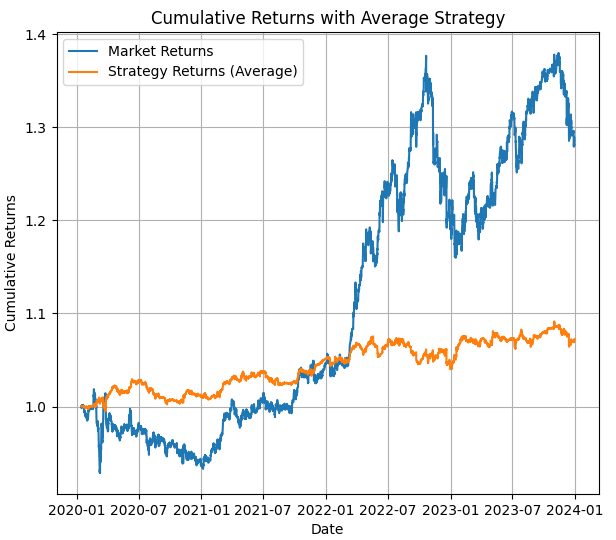
In the first image, we see the result of a backtesting with the average HMM model, you can see the price value and the strategy with HMM results for the backtesting that period.
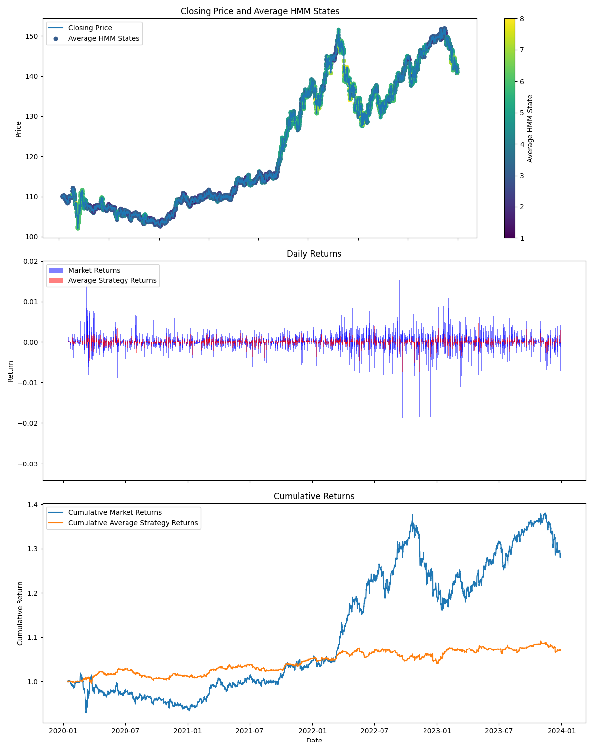
In the second image, we can see the results of the backtesting in the testing period, and a important image that shows where do the hidden states are used (you can see where they have gotten an up trend or a down trend or its ranging or neutral).
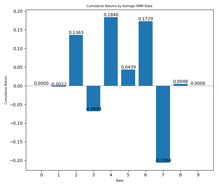
In the third image, you can see the winnings for each hidden state in bars.
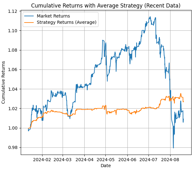
There is a fourth image with the average returns for the strategy during the period between the last date and today (this is what we should expect of the strategy in the MetaTrader 5 backtesting if we don't adjust the states).
Now that we have all this information, we can use this to select which hidden stats we will use, and we can know if a hidden state gets when its trending (with the second image) and also winning (with the bars). So with all this, we will use it to switch the states in the EA.
From the bars, we can see that the hidden states that we want to use are: 2, 3 and 7, That probably correspond to range, up trend and down trend respectively could be a high trend. We can now set up the strategy in the EA, taking into account that the other hidden states where not profitable (we can do many backtesting to try to see which is the best fit).
All python scripts have used Python 3.10.
We could add the matrices to the EA (component by component because python has a different way to show matrices), but since we don't want to work much, we will use this next script to modify the matrix to a MQl5 way that we will use for the EA. This is the EA we can use for the matrix formatting:
import re
import os

def read_file(filename):
    if not os.path.exists(filename):
        print(f"Error: The file {filename} does not exist.")
        return None
    try:
        with open(filename, "r") as file:
            return file.read()
    except Exception as e:
        print(f"Error reading the file: {str(e)}")
        return None

def parse_matrix(file_content, matrix_name):
    pattern = rf"{matrix_name}\[(\d+)\]\[(\d+)\]\s*=\s*([-+]?(?:\d*\.\d+|\d+)(?:e[-+]?\d+)?)"
    matches = re.findall(pattern, file_content)
    matrix = {}
    for match in matches:
        i, j, value = int(match[0]), int(match[1]), float(match[2])
        if i not in matrix:
            matrix[i] = {}
        matrix[i][j] = value
    return matrix

def parse_covariance_matrix(file_content):
    pattern = r"average_covariance_matrix\[(\d+)\]\[(\d+)\]\[(\d+)\]\s*=\s*([-+]?(?:\d*\.\d+|\d+)(?:e[-+]?\d+)?)"
    matches = re.findall(pattern, file_content)
    matrix = {}
    for match in matches:
        i, j, k, value = int(match[0]), int(match[1]), int(match[2]), float(match[3])
        if i not in matrix:
            matrix[i] = {}
        if j not in matrix[i]:
            matrix[i][j] = {}
        matrix[i][j][k] = value
    return matrix

def format_matrix(matrix, is_3d=False):
    if not matrix:
        return "{     };"

    formatted = "{\n"
    for i in sorted(matrix.keys()):
        if is_3d:
            formatted += "        {  "
            for j in sorted(matrix[i].keys()):
                formatted += "{" + ", ".join(f"{matrix[i][j][k]:.8e}" for k in sorted(matrix[i][j].keys())) + "}"
                if j < max(matrix[i].keys()):
                    formatted += ",\n           "
            formatted += "}"
        else:
            formatted += "        {" + ", ".join(f"{matrix[i][j]:.8f}" for j in sorted(matrix[i].keys())) + "}"
        if i < max(matrix.keys()):
            formatted += ","
        formatted += "\n"
    formatted += "     };"
    return formatted

def main():
    input_filename = "USDJPY_output.txt"
    output_filename = "formatted_matrices.txt"
    content = read_file(input_filename)

    if content is None:
        return

    print(f"Input file size: {len(content)} bytes")
    print("First 200 characters of the file:")
    print(content[:200])

    transition_matrix = parse_matrix(content, "average_transition_matrix")
    means_matrix = parse_matrix(content, "average_means_matrix")
    covariance_matrix = parse_covariance_matrix(content)

    print(f"\nElements found in the transition matrix: {len(transition_matrix)}")
    print(f"Elements found in the means matrix: {len(means_matrix)}")
    print(f"Elements found in the covariance matrix: {len(covariance_matrix)}")

    output = "Transition Matrix:\n"
    output += format_matrix(transition_matrix)
    output += "\n\nMeans Matrix:\n"
    output += format_matrix(means_matrix)
    output += "\n\nCovariance Matrix:\n"
    output += format_matrix(covariance_matrix, is_3d=True)

    try:
        with open(output_filename, "w") as outfile:
            outfile.write(output)
        print(f"\nFormatted matrices saved in '{output_filename}'")
    except Exception as e:
        print(f"Error writing the output file: {str(e)}")

    print(f"\nFirst lines of the output file '{output_filename}':")
    output_content = read_file(output_filename)
    if output_content:
        print("\n".join(output_content.split("\n")[:20]))  # Display the first 20 lines

if __name__ == "__main__":
    main()
We can also use sockets (sockets are a good way to interact with mt5 using external data) to import the matrices. You can do this as it's explained in this article: Twitter Sentiment Analysis with Sockets - MQL5 Articles and even add sentiment analysis (as explained in that article) to get better trending positions.
This script will give us a .txt that will show something similar to this:
Transition Matrix:
{
        {0.15741321, 0.07086962, 0.16785905, 0.08792403, 0.11101073, 0.05415263, 0.08019415, 0.12333382, 0.09794255, 0.04930020},
        {0.16646033, 0.11065086, 0.10447035, 0.13332935, 0.09136784, 0.08351764, 0.06722600, 0.09893912, 0.07936700, 0.06467150},
        {0.14182826, 0.15400641, 0.13617941, 0.08453877, 0.09214389, 0.04040276, 0.09065499, 0.11526167, 0.06725810, 0.07772574},
        {0.15037837, 0.09101998, 0.09552059, 0.10035540, 0.12851236, 0.05000596, 0.09542873, 0.12606514, 0.09394759, 0.06876588},
        {0.15552336, 0.08663776, 0.15694344, 0.09219379, 0.08785893, 0.08381830, 0.05572122, 0.10309824, 0.08512219, 0.09308276},
        {0.19806868, 0.11292565, 0.11482367, 0.08324432, 0.09808519, 0.06727817, 0.11549253, 0.10657752, 0.06889919, 0.03460507},
        {0.12257742, 0.11257625, 0.11910078, 0.07669820, 0.16660657, 0.04769350, 0.09667861, 0.12241177, 0.04856867, 0.08708823},
        {0.14716725, 0.12232022, 0.11135735, 0.08488571, 0.06274817, 0.07390905, 0.10742571, 0.12550373, 0.11431005, 0.05037277},
        {0.11766333, 0.11533807, 0.15497601, 0.14017237, 0.11214274, 0.04885795, 0.08394306, 0.12864406, 0.06945878, 0.02880364},
        {0.13559147, 0.07444276, 0.09785968, 0.13599698, 0.12947508, 0.06385211, 0.09042617, 0.16088280, 0.06588065, 0.04559230}
     };

Means Matrix:
{
        {0.06871601, 0.14572210, 0.05961646},
        {0.06903949, 1.05226034, -0.25687024},
        {-0.04607112, -0.00811718, 0.06488246},
        {-0.01769149, 0.63694700, 0.26965491},
        {-0.01874345, 0.58917438, -0.22484670},
        {-0.02026370, 1.09022869, 0.86790417},
        {-0.85455759, 0.48710677, 0.08980023},
        {-0.02589947, 0.84881170, 0.00453701},
        {-0.38270747, 0.86916742, -0.58792329},
        {-0.16057267, 1.17106076, 0.18531821}
     };

Covariance Matrix:
{
        {  {1.25299224e+00, -4.05453267e-02, 7.95036804e-02},
           {-4.05453267e-02, 1.63177290e-01, 1.58609858e-01},
           {7.95036804e-02, 1.58609858e-01, 8.09678270e-01}},
        {  {1.23040552e+00, 2.52108300e-02, 1.17595322e-01},
           {2.52108300e-02, 3.00175953e-01, -8.11027442e-02},
           {1.17595322e-01, -8.11027442e-02, 1.42259217e+00}},
        {  {1.76376507e+00, -7.82189996e-02, 1.89340073e-01},
           {-7.82189996e-02, 2.56222155e-01, -1.30202288e-01},
           {1.89340073e-01, -1.30202288e-01, 6.60591043e-01}},
        {  {9.08926052e-01, 3.02606081e-02, 1.03549625e-01},
           {3.02606081e-02, 2.30324420e-01, -5.46541678e-02},
           {1.03549625e-01, -5.46541678e-02, 7.40333449e-01}},
        {  {8.80590495e-01, 7.21102489e-02, 3.40982555e-02},
           {7.21102489e-02, 3.26639817e-01, -1.06663221e-01},
           {3.40982555e-02, -1.06663221e-01, 9.55477387e-01}},
        {  {3.19499555e+00, -8.63552078e-02, 5.03260281e-01},
           {-8.63552078e-02, 2.92184645e-01, 1.03141313e-01},
           {5.03260281e-01, 1.03141313e-01, 1.88060098e+00}},
        {  {3.22276957e+00, -6.37618091e-01, 3.80462477e-01},
           {-6.37618091e-01, 4.96770891e-01, -5.79521882e-02},
           {3.80462477e-01, -5.79521882e-02, 1.05061090e+00}},
        {  {2.16098355e+00, 4.02611831e-02, 3.01261346e-01},
           {4.02611831e-02, 4.83773367e-01, 7.20003108e-02},
           {3.01261346e-01, 7.20003108e-02, 1.32262495e+00}},
        {  {4.00745050e+00, -3.90316434e-01, 7.28032792e-01},
           {-3.90316434e-01, 6.01214190e-01, -2.91562862e-01},
           {7.28032792e-01, -2.91562862e-01, 1.30603500e+00}},
        {  {5.47457383e+00, -1.22088743e-02, 2.56784647e-01},
           {-1.22088743e-02, 4.65227101e-01, -2.88257686e-01},
           {2.56784647e-01, -2.88257686e-01, 1.44717234e+00}}
     };
This is the format for the matrix that we will use in the EA.
Now we have two symbols that are negatively correlated and cointegrated. We have done a HMM of one of those symbols (we just need one of those because we know both symbols are correlated), and since they are negatively correlated, when we suppose one is going to go up (with HMM) we will apply Nash and if all is correct we will sell the other symbol.
We could do this with more symbols (if they are correlated buy in the same direction or sell if they are negatively correlated).
But first, I have done a script in python to show what would be the results and to play around with the hidden states. This is the script:
import MetaTrader5 as mt5
import numpy as np
import pandas as pd
from hmmlearn import hmm
import matplotlib.pyplot as plt
from datetime import datetime

# Function to load matrices from the .txt file
def parse_matrix_block(lines, start_idx, matrix_type="normal"):
    matrix = []
    i = start_idx
    while i < len(lines) and not lines[i].strip().startswith("};"):
        line = lines[i].strip().replace("{", "").replace("}", "").replace(";", "")
        if line:  # Ensure the line is not empty
            if matrix_type == "covariance":
                # Split the line into elements
                elements = [float(x) for x in line.split(',') if x.strip()]
                matrix.append(elements)
            else:
                row = [float(x) for x in line.split(',') if x.strip()]  # Filter out empty values
                matrix.append(row)
        i += 1
    return np.array(matrix), i

def load_matrices(file_path):
    with open(file_path, 'r') as file:
        lines = file.readlines()

    transition_matrix = []
    means_matrix = []
    covariance_matrix = []

    i = 0
    while i < len(lines):
        line = lines[i].strip()

        if line.startswith("Transition Matrix:"):
            transition_matrix, i = parse_matrix_block(lines, i + 1)
            i += 1  # Move forward to avoid repeating the same block

        elif line.startswith("Means Matrix:"):
            means_matrix, i = parse_matrix_block(lines, i + 1)
            i += 1

        elif line.startswith("Covariance Matrix:"):
            covariance_matrix = []
            i += 1
            while i < len(lines) and not lines[i].strip().startswith("};"):
                block, i = parse_matrix_block(lines, i, matrix_type="covariance")
                covariance_matrix.append(block)
                i += 1
            covariance_matrix = np.array(covariance_matrix)
            covariance_matrix = covariance_matrix.reshape(-1, 3, 3)

        i += 1

    return transition_matrix, means_matrix, covariance_matrix

# Load the matrices from the .txt file
transition_matrix, means_matrix, covariance_matrix = load_matrices('formatted_matrices.txt')

# Connect to MetaTrader 5
if not mt5.initialize():
    print("initialize() failed, error code =", mt5.last_error())
    quit()

# Set parameters to retrieve data
symbol = "USDJPY"  # You can change to your desired symbol
timeframe = mt5.TIMEFRAME_H4  # You can change the timeframe
start_date = datetime(2024, 1, 1)
end_date = datetime.now()

# Load data from MetaTrader 5
rates = mt5.copy_rates_range(symbol, timeframe, start_date, end_date)
mt5.shutdown()

# Convert the data to a pandas DataFrame
data = pd.DataFrame(rates)
data['time'] = pd.to_datetime(data['time'], unit='s')
data.set_index('time', inplace=True)

# Use only the closing prices column
prices = data['close'].values.reshape(-1, 1)

# Create and configure the HMM model
n_components = len(transition_matrix)
model = hmm.GaussianHMM(n_components=n_components, covariance_type="full")
model.startprob_ = np.full(n_components, 1/n_components)  # Initial probabilities
model.transmat_ = transition_matrix
model.means_ = means_matrix
model.covars_ = covariance_matrix

# Fit the model using the loaded prices
model.fit(prices)

# Predict hidden states
hidden_states = model.predict(prices)

# Manual configuration of states
bullish_states = [2,4,5,6,8]  # States considered bullish
bearish_states = [1,3,7]  # States considered bearish
exclude_states = [0,9]  # States to exclude (neither buy nor sell)

# HMM strategy:
hmm_returns = np.zeros_like(prices)
for i in range(1, len(prices)):
    if hidden_states[i] in bullish_states:  # Buy if the state is bullish
        hmm_returns[i] = prices[i] - prices[i-1]
    elif hidden_states[i] in bearish_states:  # Sell if the state is bearish
        hmm_returns[i] = prices[i-1] - prices[i]
    # If the state is in exclude_states, do nothing

# Buy and hold strategy (holding)
holding_returns = prices[-1] - prices[0]

# Plot results
plt.figure(figsize=(7, 8))
plt.plot(data.index, prices, label='Price of '+str(symbol), color='black', linestyle='--')
plt.plot(data.index, np.cumsum(hmm_returns), label='HMM Strategy', color='green')
plt.axhline(holding_returns, color='blue', linestyle='--', label='Buy and Hold Strategy (Holding)')
plt.title('Backtesting Comparison: HMM vs Holding and Price')
plt.legend()
plt.savefig("playground.png")

# Print accumulated returns of both strategies
print(f"Accumulated returns of the HMM strategy: {np.sum(hmm_returns)}")
print(f"Accumulated returns of the Holding strategy: {holding_returns[0]}")
Let's take a look at this script. It opens the txt with the matrices, downloads the data from MetaTrader 5 for that symbol and uses data from the last date we used in the other scripts, till today, to see how the hmm works. Results are shown in a .png, and we can change the states. Let's see what are the results using all the states as the second script tells us to use:
From the second script:
Description of Hidden States:
State 0: Not present (State ID: 0)
State 1: Downtrend (State ID: 1)
State 2: Uptrend (State ID: 2)
State 3: Downtrend (State ID: 3)
State 4: Uptrend (State ID: 4)
State 5: Uptrend (State ID: 5)
State 6: Uptrend (State ID: 6)
State 7: Downtrend (State ID: 7)
State 8: Uptrend (State ID: 8)
State 9: Not present (State ID: 9)
Here is what it shows:
Accumulated returns of the HMM strategy: -1.0609999999998365
Accumulated returns of the Holding strategy: 5.284999999999997
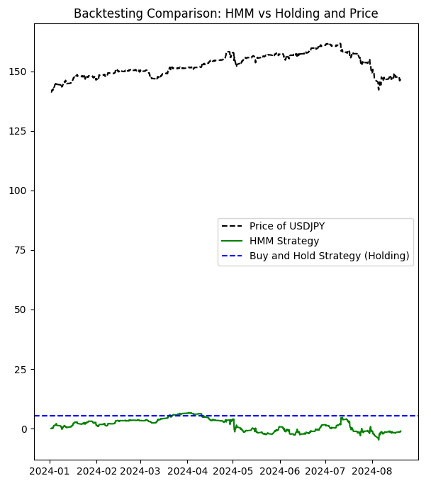
As you can see, this strategy is not really good. So, let's play around with the hidden states (that we will choose using the bar chart, we will exclude the seventh state):
# Manual configuration of states
bullish_states = [2,4,5,6,8]  # States considered bullish
bearish_states = [1,3]  # States considered bearish
exclude_states = [0,7,9]  # States to exclude (neither buy nor sell)
Accumulated returns of the HMM strategy: 7.978000000000122
Accumulated returns of the Holding strategy: 5.284999999999997
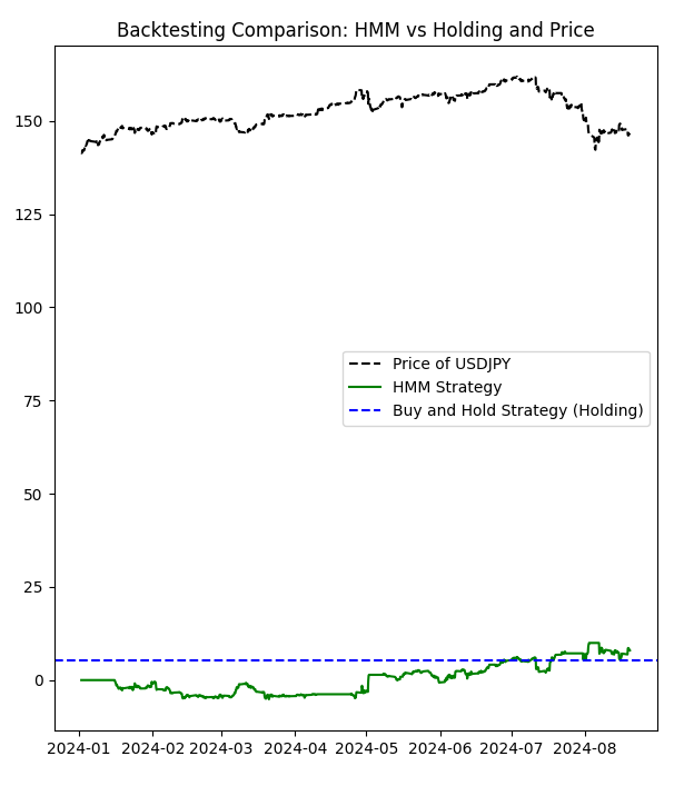
We have learned from this that when not using the worst hidden states, we can have a more profitable strategy.
Once again, also applying deep learning to this could help more detect patterns of the initial symbol (in this case USDJPY). Perhaps, we might experiment with this some other time.
Implementation in MQL5
The Nash Expert Advisor (EA) is a sophisticated algorithmic trading system designed for the MetaTrader 5 platform. At its core, the EA employs a multi-strategy approach, incorporating Hidden Markov Models (HMM), Log-Likelihood analysis, Trend Strength evaluation, and Nash Equilibrium concepts to make trading decisions in the foreign exchange market.
The EA begins by initializing crucial parameters and indicators. It sets up Essential Moving Averages (EMAs), Relative Strength Index (RSI), Average True Range (ATR), and Bollinger Bands. These technical indicators form the foundation for the EA's market analysis. The initialization process also involves setting up the Hidden Markov Model parameters, which are central to the EA's predictive capabilities.
One of the EA's key features is its market regime detection system. This system utilizes both HMM and Log-Likelihood methods to classify the current market state into three categories: Uptrend, Downtrend, or Not Present (neutral). The regime detection process involves complex calculations of emission probabilities and state transitions, providing a nuanced view of market conditions.
The EA implements four distinct trading strategies: HMM-based, Log-Likelihood-based, Trend Strength, and Nash Equilibrium. Each strategy generates its own trading signal, which is then weighted and combined to form a comprehensive trading decision. The Nash Equilibrium strategy, in particular, aims to find an optimal balance between the other strategies, potentially leading to more robust trading decisions.
Risk management is a critical aspect of the Nash EA. It incorporates features such as dynamic lot sizing based on account balance and strategy performance, stop-loss and take-profit levels, and a trailing stop mechanism. These risk management tools aim to protect capital while allowing for potential profits in favorable market conditions.
The EA also includes a backtesting functionality, allowing traders to evaluate its performance over historical data. This feature calculates various performance metrics for each strategy, including profit, total trades, winning trades, and win rate. Such comprehensive testing capabilities enable traders to fine-tune the EA's parameters for optimal performance.
In its main operational loop, the Nash EA processes market data on each new price bar. It recalculates market regimes, updates strategy signals, and makes trading decisions based on the collective output of all enabled strategies. The EA is designed to open positions in pairs, potentially trading both the primary symbol and EURCHF simultaneously, which could be part of a hedging or correlation-based strategy.
Finally, the EA includes robust error handling and logging features. It continually checks for valid indicator values, ensures that trading is allowed by the terminal and expert settings, and provides detailed logs of its operations and decision-making process. This level of transparency allows for easier debugging and performance analysis.
We will now look at some important functions and Nash's equilibria:
The main functions used to implement the Nash equilibrium concept in this Expert Advisor (EA) are:
- CalculateStrictNashEquilibrium()
This is the primary function for calculating the strict Nash equilibrium. Here's its implementation:
void CalculateStrictNashEquilibrium()
{
   double buySignal = 0;
   double sellSignal = 0;

   // Sum the weighted signals of the enabled strategies
   for(int i = 0; i < 3; i++) // Consider only the first 3 strategies for Nash equilibrium
   {
      if(strategies[i].enabled)
      {
         buySignal += strategies[i].weight * (strategies[i].signal > 0 ? 1 : 0);
         sellSignal += strategies[i].weight * (strategies[i].signal < 0 ? 1 : 0);
      }
   }

   // If there's a stronger buy signal than sell signal, set Nash Equilibrium signal to buy
   if(buySignal > sellSignal)
   {
      strategies[3].signal = 1; // Buy signal
   }
   else if(sellSignal > buySignal)
   {
      strategies[3].signal = -1; // Sell signal
   }
   else
   {
      // If there's no clear signal, force a decision based on an additional criterion
      double closePrice = iClose(_Symbol, PERIOD_CURRENT, 0);
      double openPrice = iOpen(_Symbol, PERIOD_CURRENT, 0);
      strategies[3].signal = (closePrice > openPrice) ? 1 : -1;
   }
}
Explanation:
- This function calculates buy and sell signals based on the weighted signals of the first three strategies.
- It compares the buy and sell signals to determine the Nash equilibrium action.
- If the signals are equal, it makes a decision based on the current price direction.
- SimulateTrading()
While not exclusively for Nash equilibrium, this function implements the trading logic that includes the Nash equilibrium:
void SimulateTrading(MarketRegime actualTrend, datetime time, string symbol)
{
   double buySignal = 0;
   double sellSignal = 0;

   for(int i = 0; i < ArraySize(strategies); i++)
   {
      if(strategies[i].enabled)
      {
         if(strategies[i].signal > 0)
            buySignal += strategies[i].weight * strategies[i].signal;
         else if(strategies[i].signal < 0)
            sellSignal -= strategies[i].weight * strategies[i].signal;
      }
   }

   // ... (code to simulate trades and calculate profits)
}
Explanation:
- This function simulates trading based on signals from all strategies, including the Nash equilibrium strategy.
- It calculates weighted buy and sell signals for all enabled strategies.
- OnTick()
In the OnTick() function, the logic to execute trades based on Nash equilibrium is implemented:
void OnTick()
{
   // ... (other code)

   // Check if the Nash Equilibrium strategy has generated a signal
   if(strategies[3].enabled && strategies[3].signal != 0)
   {
      if(strategies[3].signal > 0)
      {
         OpenBuyOrder(strategies[3].name);
      }
      else if(strategies[3].signal < 0)
      {
         OpenSellOrder(strategies[3].name);
      }
   }

   // ... (other code)
}
Explanation:
- This function checks if the Nash equilibrium strategy (which is the 3rd strategy in the strategies array) is enabled and has generated a signal.
- If there's a buy signal (signal > 0), it opens a buy order.
- If there's a sell signal (signal < 0), it opens a sell order.
In summary, the Nash equilibrium is implemented as one of the trading strategies in this EA. The CalculateStrictNashEquilibrium() function determines the Nash equilibrium signal based on the signals from other strategies. This signal is then used in the OnTick() function to make trading decisions. The implementation seeks to find a balance between different strategies to make more robust trading decisions.
This approach to implementing Nash equilibrium in a trading strategy is an interesting application of game theory to financial markets. It attempts to find an optimal strategy by considering the interactions between different trading signals, which is analogous to finding an equilibrium in a multi-player game where each "player" is a different trading strategy.
DetectMarketRegime Function: This function is crucial for the EA's decision-making process. It analyzes current market conditions using technical indicators and complex statistical models to determine the market regime.
void DetectMarketRegime(MarketRegime &hmmRegime, MarketRegime &logLikelihoodRegime)
{
    // Calculate indicators
    double fastEMA = iMAGet(fastEMAHandle, 0);
    double slowEMA = iMAGet(slowEMAHandle, 0);
    double rsi = iRSIGet(rsiHandle, 0);
    double atr = iATRGet(atrHandle, 0);
    double price = SymbolInfoDouble(_Symbol, SYMBOL_BID);

    // Calculate trend strength and volatility ratio
    double trendStrength = (fastEMA - slowEMA) / slowEMA;
    double volatilityRatio = atr / price;

    // Normalize RSI
    double normalizedRSI = (rsi - 50) / 25;

    // Calculate features for HMM
    double features[3] = {trendStrength, volatilityRatio, normalizedRSI};

    // Calculate log-likelihood and HMM likelihoods
    double logLikelihood[10];
    double hmmLikelihoods[10];
    CalculateLogLikelihood(features, symbolParams.emissionMeans, symbolParams.emissionCovs);
    CalculateHMMLikelihoods(features, symbolParams.emissionMeans, symbolParams.emissionCovs, symbolParams.transitionProb, 10, hmmLikelihoods);

    // Determine regimes based on maximum likelihood
    int maxLogLikelihoodIndex = ArrayMaximum(logLikelihood);
    int maxHmmLikelihoodIndex = ArrayMaximum(hmmLikelihoods);

    logLikelihoodRegime = InterpretRegime(maxLogLikelihoodIndex);
    hmmRegime = InterpretRegime(maxHmmLikelihoodIndex);


    // ... (confidence calculation code)
}
This function combines technical indicators with Hidden Markov Models and Log-Likelihood analysis to determine the current market regime. It's a sophisticated approach to market analysis, providing a nuanced view of market conditions.
CalculateStrategySignals Function: This function calculates trading signals for each of the EA's strategies based on the current market regime and technical indicators.
void CalculateStrategySignals(string symbol, datetime time, MarketRegime hmmRegime, MarketRegime logLikelihoodRegime)
{
    if(strategies[0].enabled) // HMM Strategy
    {
        CalculateHMMSignal();
    }

    if(strategies[1].enabled) // LogLikelihood Strategy
    {
        CalculateLogLikelihoodSignal();
    }

    if(strategies[2].enabled) // Trend Strength
    {
        double trendStrength = CalculateTrendStrength(PERIOD_CURRENT);
        strategies[2].signal = NormalizeTrendStrength(trendStrength);
    }

    if(strategies[3].enabled) // Nash Equilibrium
    {
        CalculateStrictNashEquilibrium();
    }
}
This function calculates signals for each enabled strategy, integrating various analytical methods to form a comprehensive trading decision.
SimulateTrading Function: This function simulates trading based on the calculated signals and updates the performance metrics of each strategy.
void SimulateTrading(MarketRegime actualTrend, datetime time, string symbol)
{
    double buySignal = 0;
    double sellSignal = 0;

    for(int i = 0; i < ArraySize(strategies); i++)
    {
        if(strategies[i].enabled)
        {
            if(strategies[i].signal > 0)
                buySignal += strategies[i].weight * strategies[i].signal;
            else if(strategies[i].signal < 0)
                sellSignal -= strategies[i].weight * strategies[i].signal;
        }
    }

    // Simulate trade execution and calculate profits
    // ... (trade simulation code)

    // Update strategy performance metrics
    // ... (performance update code)
}
This function is crucial for backtesting and evaluating the EA's performance. It simulates trades based on the calculated signals and updates each strategy's performance metrics.
CalculateHMMLikelihoods Function: This function calculates the likelihoods of different market states using the Hidden Markov Model.
void CalculateHMMLikelihoods(const double &features[], const double &means[], const double &covs[], const double &transitionProb[], int numStates, double &hmmLikelihoods[])
{
    // Initialize and calculate initial likelihoods
    // ... (initialization code)

    // Forward algorithm to calculate HMM likelihoods
    for(int t = 1; t < ArraySize(features) / 3; t++)
    {
        // ... (HMM likelihood calculation code)
    }

    // Normalize and validate likelihoods
    // ... (normalization and validation code)
}
This function implements the forward algorithm of Hidden Markov Models to calculate the likelihood of different market states. It's a sophisticated method for predicting market behavior based on observed features.
These functions form the core of the Nash Expert Advisor's analytical and decision-making processes. The EA's strength lies in its combination of traditional technical analysis with advanced statistical methods like Hidden Markov Models and Nash Equilibrium concepts. This multi-strategy approach, coupled with robust backtesting and risk management features, makes it a potentially powerful tool for algorithmic trading in the forex market.
The most important aspect of this EA is its adaptive nature. By continuously evaluating market regimes and adjusting strategy weights based on performance, it aims to maintain effectiveness across varying market conditions. However, it's crucial to note that while sophisticated, such systems require careful monitoring and periodic recalibration to ensure they remain effective in ever-changing market environments.
Results
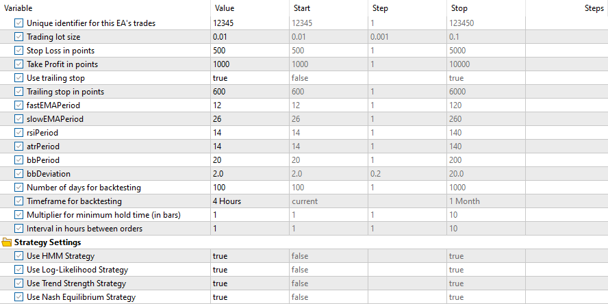
With these setings

and these Inputs
Results for all the strategies were as follows:
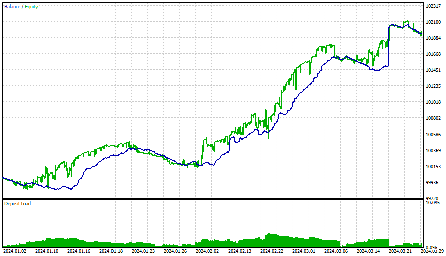
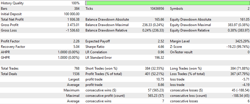
After this period, the winnings slowed down, and optimization should have been done for every 3 months (with all this starting conditions). The strategies are simple, and used a trailing stop (that is very simple and fixed). Better results can be obtained with more optimizations, with newer matrices and with better and more sophisticated strategies. We must also consider adding sentiment analysis and deep learning to this EA without forgetting whats said before.
All strategies need Nash to work.
Conclusion
The intersection of game theory and trading presents exciting opportunities for enhancing market strategies. By applying Nash's equilibrium theory, traders can make more calculated decisions, considering the potential actions of others in the market. This article has outlined how to implement these concepts using Python and MetaTrader 5, offering a powerful toolset for those looking to elevate their trading approach. As markets continue to evolve, integrating mathematical theories like Nash Equilibrium could be a key differentiator in achieving consistent success in trading.
I hope you enjoyed reading this article or replaying the article and I hope this will be helpful for your own EA, this is a interesting subject and I hope it reached your expectancy and you like it as much as I liked producing it. Neural Network in Practice: Secant Line
 MQL5 Wizard Techniques you should know (Part 34): Price-Embedding with an Unconventional RBM
 Automating Trading Strategies with Parabolic SAR Trend Strategy in MQL5: Crafting an Effective Expert Advisor
 Creating an MQL5-Telegram Integrated Expert Advisor (Part 3): Sending Chart Screenshots with Captions from MQL5 to Telegram
- Free trading apps
- Over 8,000 signals for copying
- Economic news for exploring financial markets
You agree to website policy and terms of use
I spent a whole day trying to figure out your code. The instructions in the Python section were clear, and I was able to replicate almost the exact same backtest results as yours. However, the later part of the article was quite obscure, with little explanation of the logic behind pairs trading statistical arbitrage and how exactly game theory was applied.
Here are two examples of problems I encountered with your code:
The isPositiveDefinite() function is intended to check if a single 3×3 covariance matrix is positive definite. However, in InitializeHMM , you pass the entire emissionCovs array to isPositiveDefinite() instead of individual 3×3 matrices.
The way you quantify the strategy signal is also flawed. Both the strategy log-likelihood and strategy trend output the exact same signal, while the HMM signal seems irrelevant. Turning off the HMM signal literally doesn’t change anything, yet your entire article centers around the HMM implementation.
Your strategy is based on arbitrage, and lot size should be a crucial part of it. You do have a calculateLotSize() function, but it isn’t used in your demonstration. And do you seriously believe retail traders will be trading almost every single 4hr candle? The later backtest result wasn’t profitable, yet you claim it should be optimized every couple of months. But what exactly would be optimized? The indicator period?
I’ve read many of your articles, and they’re mostly interesting. However, I think this one is not well-constructed and I would advise the readers to not waste too much time on this like I did. I genuinely hope you maintain the quality of your articles in the future.
I also spent a lot of time , this code is not clear, even some mistakes