MQL5 Wizard Techniques you should know (Part 34): Price-Embedding with an Unconventional RBM

Introduction

We continue these series that explore various trade setups and ideas thanks to MetaTrade-5’s rapid development and prototyping environment with the MQL5 wizard. These articles, in principle, seek to explore how else traders can set themselves apart from the pack by exploring ideas that may not be so common and could deliver an edge to the interested trader, depending on how he chooses to exploit them. So, we are into exploring here, not necessarily exploiting and the reason why an edge matters a lot is many working trade ideas that are available tend to correlate too positively with each other.

This is super when the trends are bullish and everyone is in the green however, as many would agree, diversification is what would mitigate drawdowns when trends reverse and yet simply finding inversely correlated securities is a lot harder than it seems on paper. That’s why trade entries and exits that are specific to a trader could be a better haven than simply relying on commonly used setups. With that, this article looks at the Restricted Boltzmann Machines (RBMs) when implemented with Backpropagation, as opposed to their traditional implementations of Gibbs Sampling and Contrastive Divergence.

It is argued that the reason these approaches were used to begin with was because in the mid 80s (circa 1986 when RBMs were introduced under the name Harmonium) computing costs of implementing back propagation in Boltzmann Machines, was simply not feasible. Boltzmann Machines, from which RBMs get their name, are even more complex since they do not use a bi-partite graph like RBMs but instead have intra neuron connections within a layer. These connection complexities are what biased even a simpler implementation of the Boltzmann Machines like RBMs to rely on probability Energy Based Models (EBMs) in fine-tuning parameters (weights & biases) of the network rather than having to process or deal with each parameter at a time as is practice with other neural networks and in Backpropagation.

As per Deep-AI:

Contrastive Divergence addresses the computational challenge posed by the partition function in energy-based models. The key insight behind Contrastive Divergence is that it's possible to train these models without having to calculate the full partition function. Instead, CD focuses on adjusting the model parameters so that the probability of the observed data increases while the probability of samples generated by the model decreases. 

To achieve this, Contrastive Divergence performs a Gibbs sampling procedure starting from the training data to produce samples that the model believes are likely. It then uses these samples toestimatethe gradient of the log-likelihood of the training data with respect to the model parameters. This gradient is used to update the parameters in a direction that improves the model's representation of the data.

So, in order to avoid computations for each probability, Gibbs sampling and contrastive divergence were a boon that clearly made sense. Fast-forward to today and when presented with the same problem(s) Backpropagation can certainly be a feasible option, especially when one considers that most of the AI workload is no longer borne by CPUs, but GPUs are significantly taking on these tasks and at an accelerated pace. This choice of hardware when handling Boltzmann-Machine-like networks (like the RBM) is key because even though they have only 2 layers, these layers tend to be very deep and so how the weights of each neuron are adjusted needs to be properly considered.

So then, what really are RBMs given the 2-layer limit? The short answer is a classifier, that reduces the dimensions of its input data to reveal hidden properties of the data in fewer dimensions than the input. This is an overly simplified definition, as a more diligent one would mention they are generative stochastic neural networks trained in unsupervised settings to learn the probability distribution of their input data. The findings from the input data, that are logged in the network’s hidden layer, can then be used in classification, clustering, or as input to another network.

For this article, we are exploiting the latter, taking our RBMs hidden layer values as input to a Multi-Layer-Perceptron. The overall structure of the article will in principle follow the format we have been accustomed to throughout these series.

Price-Embedding

Price-Embedding is used in the context of this article as a process very akin to word embedding; and this as some readers may know is the prerequisite step to transformer networks of large language models. Word embedding, which can be defined as the numberfication of words, when paired with self-attention, helps convert a lot of the written material that is available online into a format that neural networks can understand. We are similarly taking a leaf from this approach by making a presumption that, by default, security price data (Even though numeric) cannot be easily ‘understood’ by neural networks off the bat. And our approach for making this more understandable is by using a backpropagation trained RBM.

Now, the conversion of words to numbers is not simply about assigning a number to a word or letter, but rather it is an intricate process that involves self-attention as already mentioned above. Parallels from this, I believe, can be drawn to RBMs when one considers their bi-partite graph design.

source

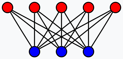
While there are no direct neuron-to-neuron connections within a layer of an RBM, these connections, which could be key in capturing the self-attention component of any input data, are made through the hidden layer. With this thesis, the hidden layer not only logs what each neuron could be redrawn as, but also what the significance of its relationships to the other neurons is.

As always, as far as traders are concerned the proof is in the pudding and so the benefits of this price-embedding can only be proven by trading results. And we are going to get to the first part of this process however it could be worth highlighting that scale of rewards one gets from word to number embedding cannot be compared to those we are looking at in the number to number embedding this is because what we are doing here is not nearly as transformational. With that, let's now consider how we reconstruct an RBM with backpropagation.

Restricted Boltzmann Machines (RBMs)

RBMs operate in two cycles that are often referred to as the positive phase and negative phase. As already mentioned they are often unsupervised (although some supervised versions have been implemented) and this means inherently that as we start and go through the training process, we do not know what the hidden properties of each tested data point ought to be. The training data has no labels (or target values).

The way RBMs keep-score therefore is by reconstructing the hidden layer values to match the input layer values in the negative phase. So, there are 2 phases, the positive phase which is similar to the forward propagation of a regular MLP provides values to the hidden layer. These hidden layer values are our objective, as they are a dimensionality reduced representation of the input data that captures properties we seek.

In propagating towards the hidden layer (the positive phase) a matrix of weights is used as is the case in neural networks; what makes RBMs special, though, is that in the negative phase, the same weights are used to reconstruct the input data. This reconstruction as mentioned is how the RBM trains unsupervised or keeps score and since we are implementing Backpropagation, the input data serves as the de-facto label (or target) to itself.

I maintain that this is still unsupervised because no additional data outside-of the training input data is required to train this RBM. In instances where supervised training was performed with RBMs, labels of ideal hidden layer values were used, and that is not what we are doing here. So, to start off, we would need to reconstruct the typical RBM functions of positive phase and negative phase. This is as follows:

//+------------------------------------------------------------------+
//|                                                                  |
//+------------------------------------------------------------------+
void C_u_rbm::GetPositive(void)
{  vector _positive = weights[0].MatMul(inputs), _output;
   _positive += biases[0];
   _positive.Activation(_output, THIS.activation);
   output = _output;
}

//+------------------------------------------------------------------+
//|                                                                  |
//+------------------------------------------------------------------+
void C_u_rbm::GetNegative(void)
{  vector _negative = output.MatMul(weights[0]), _output;
   _negative += biases[1];
   _negative.Activation(_output, THIS.activation);
   label = _output;
}

Our MQL5 class from this, ‘C_u_rbm’ inherits from another class ‘Cmlp’ that we have been using in recent articles. The construction of ‘C_u_rbm’ even though it inherits from ‘Cmlp’ needs to be customized to ensure the appropriate number of layers are in place and the relevant validation steps are covered. We perform this class’ construction as follows, as indicated in its interface:

#include <My\Cmlp-.mqh>
//+------------------------------------------------------------------+
//| Unconventional RBM that uses:                                    |
//| reconstruction-error instead of free-energy                      |
//| and back-propagation instead of contrastive divergence           |
//+------------------------------------------------------------------+
class C_u_rbm : public Cmlp
{
protected:

public:
   void              GetPositive();
   void              GetNegative();
   
   void              BackPropagate(double LearningRate = 0.1);

   double            Get(ENUM_REGRESSION_METRIC R)
   {                 return(label.RegressionMetric(inputs, R));
   }

   void              C_u_rbm(Smlp &MLP) : Cmlp(MLP)
   {  validated = false;
      int _layers =    ArraySize(MLP.arch);
      if(_layers == 2 && MLP.arch[0] > MLP.arch[1])
      {  ArrayResize(biases, _layers);
         //
         ArrayResize(gradients, _layers);
         ArrayResize(gradients_1st_moment, _layers);
         ArrayResize(gradients_2nd_moment, _layers);
         ArrayResize(sum_gradients, _layers);
         ArrayResize(sum_gradients_update, _layers);
         //
         ArrayResize(deltas, _layers);
         ArrayResize(deltas_1st_moment, _layers);
         ArrayResize(deltas_2nd_moment, _layers);
         ArrayResize(sum_deltas, _layers);
         ArrayResize(sum_deltas_update, _layers);
         //
         hidden_layers = 0;
         bool _norm_validated = true;
         for(int i = 0; i < _layers; i++)
         {  int _rows = MLP.arch[_layers - 1 - i], _columns = MLP.arch[i];
            //
            biases[i].Init(_rows);
            biases[i].Fill(MLP.initial_bias);
            //
            gradients[i].Init(_rows, _columns);
            gradients[i].Fill(0.0);
            //
            gradients_1st_moment[i].Init(_rows, _columns);
            gradients_1st_moment[i].Fill(0.0);
            gradients_2nd_moment[i].Init(_rows, _columns);
            gradients_2nd_moment[i].Fill(0.0);
            //
            sum_gradients[i].Init(_rows, _columns);
            sum_gradients[i].Fill(0.0);
            sum_gradients_update[i].Init(_rows, _columns);
            sum_gradients_update[i].Fill(0.0);
            //
            deltas[i].Init(_rows);
            deltas[i].Fill(0.0);
            deltas_1st_moment[i].Init(_rows);
            deltas_1st_moment[i].Fill(0.0);
            deltas_2nd_moment[i].Init(_rows);
            deltas_2nd_moment[i].Fill(0.0);
            sum_deltas[i].Init(_rows);
            sum_deltas[i].Fill(0.0);
            sum_deltas_update[i].Init(_rows);
            sum_deltas_update[i].Fill(0.0);
         }
         validated = true;
      }
      else
      {  printf(__FUNCSIG__ +
                " invalid network arch! Settings size is: %i, Max layer size is: %i, Min layer size is: %i, and activation is %s ",
                _layers, MLP.arch[ArrayMaximum(MLP.arch)], MLP.arch[ArrayMinimum(MLP.arch)], EnumToString(MLP.activation)
               );
      }
   };
   void              ~C_u_rbm(void) { };
};

In customizing the constructor for our class, we omitted the weights' matrix array because its size is always the total number of layers minus one, and that is what we have here. The constructor therefore dealt with what is different, firstly we are having two bias vectors even though the layers are only two. This implies we will have two delta vectors as well, with one for each bias vector. Another necessary customization is in the number of gradient matrices. Despite having only, one weights matrix, we have two gradient matrices because our backpropagation will be for the two test cycles; the positive phase and the negative phase.

This also implies that our single matrix of weights gets updated twice in each backpropagation. As always, backpropagation involves computing the deltas, then the gradients, then the updating of weights and biases with these values. We perform our backpropagation as follows:

//+------------------------------------------------------------------+
//|                                                                  |
//+------------------------------------------------------------------+
void C_u_rbm::BackPropagate(double LearningRate = 0.1)
{  
//COMPUTE DELTAS
   vector _loss = label.LossGradient(inputs, THIS.loss);
   //
   vector _negative = output.MatMul(weights[0]), _negative_derivative;
   _negative.Derivative(_negative_derivative, THIS.activation);
   deltas[1] = Hadamard(_loss, _negative_derivative);
   //
   vector _positive = weights[0].MatMul(inputs), _positive_derivative;
   _positive.Derivative(_positive_derivative, THIS.activation);
   matrix _weights;
   _weights.Copy(weights[0]);
   _weights.Transpose();
   vector _product = _weights.MatMul(deltas[1]);
   deltas[0] = Hadamard(_product, _positive_derivative);
//COMPUTE GRADIENTS
   gradients[0] = TransposeCol(deltas[0]).MatMul(TransposeRow(inputs));
   gradients[1] = TransposeCol(deltas[1]).MatMul(TransposeRow(output));
   
// UPDATE WEIGHTS AND BIASES
   for(int h = 1; h >= 0;  h--)
   {  matrix _gradients;
      _gradients.Copy(gradients[h]);
      if(h == 1)
      {  _gradients = _gradients.Transpose();
      }
      weights[0] -= LearningRate * _gradients;
      biases[h] -= LearningRate * deltas[h];
   }
}

This function therefore sums up our class that inherits from ‘Cmlp’ with all non-overridden functions of the base class still in effect. Just to clarify why we have two bias vectors, two delta vectors, two gradients matrices and only a single weights matrix is on the positive phase we encounter the weights' matrix for the first time and the product from that needs to be added to the first bias vector. This product also implies a gradient matrix needs to be captured in order to properly update the weights over this product. Over the second phase the same process gets repeated with the key difference being, as already mentioned, that we use the same weights of the positive phase.

Despite using the same weights though, a new (different) bias vector gets added to the product of the second phase and this produces our reconstruction of the input data. The difference between this reconstructed data and the original input data then defines our deltas, and this feeds into the backpropagation.

RBM in the Custom Signal Class

To build the custom signal class, we would need to reference our custom RBM class created above in a new instance of a custom signal class that we assemble into an Expert Advisor via the MQL5 wizard. There are guides here and here on this for readers who are new. And once we reference it and set it up we would have only half of our trade system because as mentioned in the introduction, we have the RBM hidden layer values of their input data serving as input to another neural network in the form of a multi-layer-perceptron (MLP). The function performed by the RBM is embedding price changes to unmask their equivalent in a smaller dimension. For our testing, our RBM is an 8-4 network, where the numbers are the sizes of the visible and hidden layers. The RBM task in my opinion leans more towards classification than regression and therefore the loss function and activation, will be categorical cross entropy and soft-sign. These could still be tweaked to be workable as classifiers, as we covered in recent articles, however we are using these settings as constants and they are not optimizable.

The functions performed by the RBM as mentioned are more aligned with embedding, and thus the function responsible for performing this in our custom signal class in named the ‘Embedder’. Its source code is shared below:

//+------------------------------------------------------------------+
//|                                                                  |
//+------------------------------------------------------------------+
void CSignalEmbedding::Embedder(vector &Extraction)
{  m_learning.rate = m_learning_rate;
   for(int i = 1; i <= m_epochs; i++)
   {  U_RBM.LearningType(m_learning, i);
      for(int ii = m_train_set; ii >= 0; ii--)
      {  vector _in, _in_new, _in_old, _out, _out_new, _out_old;
         if
         (
         _in_new.Init(__RBM_VISIBLE) && 
         _in_new.CopyRates(m_symbol.Name(), m_period, 8, ii + __MLP_OUTPUTS, __RBM_VISIBLE) && 
         _in_new.Size() == __RBM_VISIBLE &&
         _in_old.Init(__RBM_VISIBLE) && 
         _in_old.CopyRates(m_symbol.Name(), m_period, 8, ii + __MLP_OUTPUTS + 1, __RBM_VISIBLE) && 
         _in_old.Size() == __RBM_VISIBLE
         &&
         _out_new.Init(__MLP_OUTPUTS) &&
         _out_new.CopyRates(m_symbol.Name(), m_period, 8, ii, __MLP_OUTPUTS) &&
         _out_new.Size() == __MLP_OUTPUTS &&
         _out_old.Init(__MLP_OUTPUTS) &&
         _out_old.CopyRates(m_symbol.Name(), m_period, 8, ii + __MLP_OUTPUTS, __MLP_OUTPUTS) &&
         _out_old.Size() == __MLP_OUTPUTS
         )
         {  _in = _in_new - _in_old;
            _out = _out_new - _out_old;
            U_RBM.Set(_in);
            U_RBM.GetPositive();
            U_RBM.GetNegative();
            U_RBM.BackPropagate(m_learning.rate);
            Extraction = Extractor(U_RBM.output, _out, ii > 0);
         }
      }
   }
}

Our data preparation is very similar to what we had in past articles. In most Expert Advisors that are coded manually and not via the MQL5 wizard, extra steps need to be taken to ensure price data queried by the Expert Advisor is actually available on the broker’s server before signal computations are made. Usually when a wizard assembles the Expert Advisor this can be skimped, in our case though we simply use the if-clause to ensure the data we seek is actually copied in our intended vectors.

When copying data to vectors, it’s also important to keep in mind that the data is not sorted as a series, implying the highest index in the vector copied to have the latest value. There is more here on this subject. Because we have a chain arrangement where the RBM provides input to the MLP, we have elected to train the two networks almost concurrently, where at each point in the training set of the RBM we train the RBM and then follow this up by also training the MLP. This is different from first exhausting the RBM’s training session before training the MLP.

This arrangement is certainly amendable by the reader given that the complete source for this is attached at the bottom, however we adopt it because it could be more efficient given the need to train two networks, for our testing purposes. Given the almost concurrent training, we need to get the RBM input and MLP labels at the same time, and that’s why our if clauses are very lengthy.

Integrating the RBM with an MLP

So, through the training process, we update the RBM weights which allows us to process more input data and get its hidden values (aka its probability distribution). This probability distribution which we are referring to as the price-embedding are then fed to the MLP, and not the raw prior price changes. The using of this embedding is in the ‘Extractor’ function, which simply feeds forward the price embedding provided by the RBM through the MLP. As it feeds through, it also trains the MLP if a label (target value) is provided. Because training is performed up to the most recent price-changes for which they would be no label, we need to keep track of this. The tracker is the third input parameter in the ‘Extractor’ function that is the boolean ‘Train’. By default, it is true, however once we get to the end of the training set, and we have no label it gets assigned to false. The code for the ‘Extractor’ function is shared below:

//+------------------------------------------------------------------+
//|                                                                  |
//+------------------------------------------------------------------+
vector CSignalEmbedding::Extractor(vector &Embedding, vector &Labels, bool Train = true)
{  vector _extraction;
   _extraction.Init(MLP.output.Size());
   m_learning.rate = m_learning_rate;
   for(int i = 1; i <= m_epochs; i++)
   {  MLP.LearningType(m_learning, i);
      MLP.Set(Embedding);
      MLP.Forward();
      _extraction = MLP.output;
      if(Train)
      {  MLP.Get(Labels);
         MLP.Backward(m_learning, i);
      }
   }
   return(_extraction);
}

It returns a vector that we are calling ‘_extraction’ but in our case we are only interested in one value, the next price change, so it’s really a one sized vector. While the RBM is structured like a classifier by its activation function and loss function, the MLP should probably work better when structured like a regressor. This is because of its singular floating data output that can be negative. As a regressor we use soft-sign activation and the loss function is Huber. Reasons for this when dealing with regressor networks were covered in recent articles such as here, so new readers can take a look.

Both the RBM and MLP are not properly tuned for optimal performance because, for instance, they use identical initial weights and biases, plus the training is concurrent, essentially meaning one training session is used to train both networks. Alternatives to this do include having different sized training sessions for the RBM and MLP, where the MLP training is only done once the RBM training is complete. In addition, the learning rate is fixed for both networks and different formats that include adaptive learning have not been exploited. A lot of these additional adjustments and more are left to the reader to check out.

Back testing and Optimization

We do an optimization over the year 2023 for the pair GBPUSD on the daily time frame while seeking the ideal initial network weights and biases. Recall, we have a single input parameter for both these values to the two networks, which is not necessarily ideal. In addition, we are seeking the opening and closing thresholds for the ‘LongCondition’ and ‘ShortCondition’ functions of our custom signal class, plus a take profit level in points. We perform a few runs that are not exhaustive, and from them, we have the following results:

Our wizard assembled Expert Advisor can trade, however as is always the case more diligence is necessary in as far as testing over longer periods of history and following up optimizations with forward walk tests. Also, worth mentioning is that this being a neural network-based signal, the logging and saving of the network (there are 2 here) weights and biases is something the user should always plan for.

Conclusion

We have provided an RBM as a price embedder to an MLP with its optimized trade results over a single year, but how could one gauge the efficacy of ‘price-embedding’ in the context within which it is used in this article? Well the short answer is if we have another purely MLP signal that takes as inputs the raw prior price changes and is also trained like the MLP of this article to project the next price change. Setting this up is also relatively easy because the anchor classes for the MLP are similar to what we have been using, so comparative results can easily be obtained.

We have also paired an RBM that feeds into an MLP and not the other way around. This, I feel, is a better way for these two types of neural networks to work together (a classifier and a regressor). Regressors often but not always are outputting a single floating-point value (that can be negative) and by taking in ‘classified’ inputs this pairing could be justified. Going forward this arrangement can be expanded, not by stacking the RBMs since they exploit depth, but by having them lined in parallel as inputs to transformer-cued regressor networks. The classifiers with their depth I feel are better built for ‘specialization’ than regressor networks.

Also, as a final note we have simply looked to classify price changes as the ‘price-embedding’ however different financial data and time series can also be considered when seeking ‘price-embedding’ data to an MLP. These could include candle stick price patterns, price indicator values, economic calendar news data etc. The performance and test results for each of these is bound to vary a lot, as one would expect, and so it’s up to the reader to find and customize what would work best with the way they view the markets.