Time series clustering in causal inference

Introduction

• What is clustering
• Applying clustering in causal inference
• Matching using clustering
• Determining heterogeneous treatment effect
• Defining market modes

Volatility clustering:

• Code
• Rating of algorithms
• Model input parameters

Matching trades using clustering:

• Code
• Algorithm
• Accounting for data heterogeneity
• Results
• Conclusion

Introduction

Clustering is a machine learning technique that divides a dataset into groups of objects (clusters) so that objects within the same cluster are similar to each other, and objects from different clusters are different. Clustering can help in revealing the data structure, identifying hidden patterns and grouping objects based on their similarity.

Clustering can be used in causal inference. One way to apply clustering in this context is to identify groups of similar objects or events that can be associated with a particular cause. Once data is clustered, relationships between clusters and causes can be analyzed to identify potential cause-and-effect relationships.

In addition, clustering can help identify groups of objects that may be subject to the same effects or have common causes, which can also be useful in analyzing cause-and-effect relationships.

The use of clustering in causal inference can be especially useful for analyzing data and identifying potential cause-and-effect relationships. Within this article, we will consider how clustering can be utilized in this context:

1. Identifying groups of similar objects: Clustering allows you to identify groups of objects that have similar characteristics or behavior. You can then analyze these groups and look for common causes or factors that may be associated with them.
2. Determining cause-and-effect relationships: Once the data has been divided into clusters, relationships between clusters can be explored and potential cause-and-effect relationships can be identified. For example, if a certain cluster of objects exhibits a certain behavior or characteristics, analysis can be done to find out what factors may be responsible for it.
3. Finding hidden patterns: Clustering can help reveal hidden patterns in data that may be related to cause-and-effect relationships. By analyzing the structure of clusters and identifying common object characteristics within them, it is possible to discover factors that may play a key role in the occurrence of certain phenomena.
4. Predicting future events: Once clusters and cause-and-effect relationships have been identified, the knowledge gained can be used to predict future events or trends. Based on data analysis and identified patterns, you can make assumptions about what factors may influence future events and what measures can be taken to manage them.

Clustering can be used for matching in causal inference. Matching is the process of matching objects from different datasets based on their similarity or compliance with certain criteria. In the context of causal inference, matching can be used to establish relationships between causes and effects, and to identify common characteristics or factors that may be responsible for certain phenomena.

In matching, clustering can be useful for the following:

1. Grouping of objects: Clustering allows you to divide a data set into groups of objects that have similar characteristics or behavior. After this, you can run matching within each cluster to find matches between objects and establish connections between them.
2. Similarity identification: Once objects have been divided into clusters, similarities between objects within each cluster can be examined and used for matching. For example, if a certain cluster of objects exhibits similar behavior or characteristics, matching can be done to find common factors that may be associated with these objects.
3. Noise reduction: Clustering can help reduce noise in data and highlight major groups of objects, making the matching process easier. By dividing data into clusters, you can focus on the most significant and similar objects, which improves the quality of matching and allows you to identify clearer cause-and-effect relationships.

As a result, time series clustering can help identify heterogeneous treatment effects, that is, differences in effects in different groups of time series. In the context of time series analysis where classification or forecasting is performed, the heterogeneous treatment effect means that the behavior of the time series may vary depending on its characteristics or other factors.

Thus, by clustering time series, the following effects can be achieved:

1. Grouping time series: Clustering allows time series to be divided into groups based on their characteristics, trends, or other factors. The behavior of each group can then be examined separately to determine whether there are differences in prediction or classification between different time series clusters.
2. Identifying subgroups with different effects: By clustering time series, subgroups with different behavior or trajectories of change can be identified. This allows researchers to determine what characteristics or factors may influence classification or prediction results and identify subsets of time series that may require different analysis approaches.
3. Personalization of models: Using clustering results and identified subgroups of time series with different behavior, you can personalize classification or forecasting models and select optimal strategies for each group. This allows you to improve forecast and classification accuracy and adapt models to different types of time series.

Clustering can also be viewed in terms of identifying market regimes, for example based on volatility.

Market volatility analysis is a key tool for investors and traders as it allows them to understand the current state of the market and make informed decisions based on expected price movements. In the context of financial analysis, volatility-based clustering algorithms help highlight different market "regimes" that may indicate different trends, phases of consolidation, or periods of high uncertainty.

How does the clustering algorithm work in problems of determining market regimes based on volatility:

• Data Preparation: The raw price volatility time series for assets are preprocessed, including calculating volatility based on the standard deviation of prices or variations in the price distribution.
• Applying a clustering algorithm: The clustering algorithm is then applied to the volatility data to identify hidden structures and groups of market regimes. Various methods can be used as a clustering algorithm, such as K-Means, DBSCAN, or algorithms specifically designed for time series analysis, such as algorithms that take into account time dependencies.
• Interpretation of the results: The resulting clusters represent different market regimes that can be interpreted in the context of trading strategies. For example, clusters with low volatility may correspond to periods of sideways trend, while clusters with high volatility may indicate market spikes or trend changes.

Advantages of the clustering algorithm in problems of determining market regimes based on volatility:

• Determining the market structure: Clustering algorithms make it possible to highlight the market structure and identify hidden modes, which helps investors and traders understand the current state of the market.
• Automation of analysis: the use of clustering algorithms allows you to automate the process of analyzing market volatility and identifying different modes, which saves time and reduces the likelihood of human errors.
• Decision support: Identifying market patterns based on volatility helps predict future price movements and make informed trading and investing decisions.

Disadvantages of the clustering algorithm in problems of determining market regimes based on volatility:

• Sensitivity to parameter selection: Clustering results may depend on the selection of algorithm parameters, such as the number of clusters or distance metric, which requires careful tuning.
• Limitations of the algorithms: Some clustering algorithms may not be efficient when processing large amounts of data or may not take into account time dependencies.

Types of clustering algorithms

We can use different clustering algorithms for our tasks. The main types of clustering are available as ready-made libraries implemented in Python. So, the best way to start experimenting with clustering is to use the libraries, since you don't have to implement each algorithm from scratch. This significantly speeds up the process of setting up and conducting the experiment.

We will briefly look at the main clustering algorithms that may be useful to us and will then apply them in our tasks.

• K-Means stands out for its simplicity and efficiency but has limitations such as dependence on initial conditions and the need to know the number of clusters.
• Affinity Propagation does not require pre-determining the number of clusters and works well with data of various shapes but can be computationally complex.
• Mean Shift is capable of detecting clusters of arbitrary shape and does not require specifying the number of clusters. It can be computationally expensive when working with large amounts of data.
• Spectral Clustering is suitable for data with nonlinear structures and is universal. However, it can be difficult to tune parameters and computationally expensive.
• Agglomerative Clustering creates hierarchical clusters and is suitable for dealing with an unknown number of clusters.
• GMM offers a probabilistic approach to clustering, allowing the modeling of clusters with different shapes and densities.
• HDBSCAN and BIRCH both provide efficient handling of large amounts of data and automatic determination of the number of clusters, but also have their drawbacks, such as computational complexity and sensitivity to parameters.

Implementation of time series clustering (volatility clustering)

We are interested in the possibility of clustering financial time series both as a means to determine market regimes and as a means to match and determine the heterogeneous treatment effect. We begin by attempting to cluster market regimes.

The following code trains the meta-learning model and then trains the final model and meta-model based on the results of clustering, which is based on the volatility of financial data:

def meta_learner(models_number: int, 
                 iterations: int, 
                 depth: int, 
                 bad_samples_fraction: float, 
                 n_clusters: int, 
                 algorithm: int) -> pd.DataFrame:
    
    dataset = get_labels(get_prices())
    data = dataset[(dataset.index < FORWARD) & (dataset.index > BACKWARD)].copy()
    X = data[data.columns[1:-2]]
    X = X.loc[:, ~X.columns.str.contains('std')]
    meta_X = data.loc[:, data.columns.str.contains('std')]
    y = data['labels']

    B_S_B = pd.DatetimeIndex([])
    for i in range(models_number):
        X_train, X_val, y_train, y_val = train_test_split(
            X, y, train_size = 0.5, test_size = 0.5, shuffle = True)
        
        # learn debias model with train and validation subsets
        meta_m = CatBoostClassifier(iterations = iterations,
                                depth = depth,
                                custom_loss = ['Accuracy'],
                                eval_metric = 'Accuracy',
                                verbose = False,
                                use_best_model = True)
        
        meta_m.fit(X_train, y_train, eval_set = (X_val, y_val), plot = False)
        
        coreset = X.copy()
        coreset['labels'] = y
        coreset['labels_pred'] = meta_m.predict_proba(X)[:, 1]
        coreset['labels_pred'] = coreset['labels_pred'].apply(lambda x: 0 if x < 0.5 else 1)
        
        # add bad samples of this iteration (bad labels indices)
        diff_negatives = coreset['labels'] != coreset['labels_pred']
        B_S_B = B_S_B.append(diff_negatives[diff_negatives == True].index)

    to_mark = B_S_B.value_counts()
    marked_idx = to_mark[to_mark > to_mark.mean() * bad_samples_fraction].index
    data.loc[data.index.isin(marked_idx), 'meta_labels'] = 0.0


    if algorithm==0:
        data['clusters'] = KMeans(n_clusters=n_clusters).fit(meta_X).labels_
    elif algorithm==1:
        data['clusters'] = AffinityPropagation().fit(meta_X).predict(meta_X)
    elif algorithm==2:
        data['clusters'] = SpectralClustering(n_clusters=n_clusters, assign_labels='discretize', random_state=0).fit_predict(meta_X)
    elif algorithm==3:
        data['clusters'] = MeanShift().fit_predict(meta_X)
    elif algorithm==4:
        data['clusters'] = AgglomerativeClustering(n_clusters=n_clusters).fit_predict(meta_X)
    elif algorithm==5:
        data['clusters'] = mixture.GaussianMixture(n_components=n_clusters, covariance_type='full').fit(meta_X).predict(meta_X)
    elif algorithm==6:
        data['clusters'] = HDBSCAN(min_cluster_size=150).fit_predict(meta_X)
    elif algorithm==7:
        data['clusters'] = Birch(threshold=0.01, n_clusters=n_clusters).fit_predict(meta_X)
    return data[data.columns[1:]]

Function description:

The meta_learner function is designed to meta-train a classification model to identify and correct mislabeled samples in a dataset. It uses an ensemble of CatBoostClassifier models to identify such samples and applies clustering algorithms to further process the data. Here is a more detailed description of the process:

1. Preparing the data: The function begins by retrieving a dataset that is filtered by timestamps (excluding data from certain periods). Next, the data is divided into features (X), meta-features (meta_X) based on standard deviations, and target labels (y).

2. Initializing the variable: An empty date index B_S_B is created to store indexes of mislabeled samples.

3. Training models and identifying incorrect labels: for each of the models_number models, the data is divided into training and validation sets. Then the CatBoostClassifier model is trained with the given parameters. Once trained, the model is used to predict labels on the entire set of features X. By comparing the predicted labels with the original ones, the function identifies incorrectly labeled samples and adds their indexes to B_S_B.

4. Labeling bad samples: After training all models, the function analyzes the indexes of bad samples stored in B_S_B and flags those that occur more frequently than determined by bad_samples_fraction, marking them as 0.0 in the column meta_labels in the source data.

5. Clustering: depending on the value of the 'algorithm' parameter, the function applies one of the clustering algorithms to meta-features (meta_X) and adds the resulting cluster labels to the source data.

6. Returning a result: The function returns an updated dataset with labels and assigned clusters.

This approach allows not only to identify and correct errors in data labels, but also to group data for further analysis or model training, which can be especially useful in problems where there are a significant number of incorrectly labeled samples.

The training function for the final models looks like this:

def fit_final_models(dataset) -> list:
    # features for model\meta models. We learn main model only on filtered labels 
    X, X_meta = dataset[dataset['meta_labels']==1], dataset[dataset.columns[:-3]]
    X = X[X.columns[:-3]]
    X = X.loc[:, ~X.columns.str.contains('std')]
    X_meta = X_meta.loc[:, X_meta.columns.str.contains('std')]
    
    # labels for model\meta models
    y, y_meta = dataset[dataset['meta_labels']==1], dataset[dataset.columns[-1]]
    y = y[y.columns[-3]]
    
    y = y.astype('int16')
    y_meta = y_meta.astype('int16')

    # train\test split
    train_X, test_X, train_y, test_y = train_test_split(
        X, y, train_size=0.8, test_size=0.2, shuffle=True)
    
    train_X_m, test_X_m, train_y_m, test_y_m = train_test_split(
        X_meta, y_meta, train_size=0.8, test_size=0.2, shuffle=True)

    # learn main model with train and validation subsets
    model = CatBoostClassifier(iterations=200,
                               custom_loss=['Accuracy'],
                               eval_metric='Accuracy',
                               verbose=False,
                               use_best_model=True,
                               task_type='CPU')
    model.fit(train_X, train_y, eval_set=(test_X, test_y),
              early_stopping_rounds=25, plot=False)
    
    # learn meta model with train and validation subsets
    meta_model = CatBoostClassifier(iterations=100,
                                    custom_loss=['F1'],
                                    eval_metric='F1',
                                    verbose=False,
                                    use_best_model=True,
                                    task_type='CPU')
    meta_model.fit(train_X_m, train_y_m, eval_set=(test_X_m, test_y_m),
              early_stopping_rounds=15, plot=False)
    
    R2 = test_model([model, meta_model])
    if math.isnan(R2):
        R2 = -1.0
        print('R2 is fixed to -1.0')
    print('R2: ' + str(R2))
    return [R2, model, meta_model]

The fit_final_models function is designed to train the main and meta models on the provided dataset. Here is a detailed description of its operation:

1. Data preparation:

• The function selects from the dataset the rows where meta_labels is equal to 1 to train the main model (X, y).
• All rows of the dataset (X_meta, y_meta) are used to train the meta-model.
• Columns containing 'std' in the name, as well as the last three columns, are excluded from the features for training the main model.
• For the meta-model, the function only uses the features that contain 'std' in the name.
• The target variable (y) for the main model is taken from the third column from the end and cast to type int16.
• The target variable for the meta-model (y_meta) is taken from the last column and is also cast to int16.

2. Dividing the data into training and test samples:

• For the main model and meta-model, the data is divided into training and test samples in a ratio of 80% to 20%.

3. Basic model training:

• We use the CatBoostClassifier classifier with 200 iterations, the 'Accuracy' loss function and the 'Accuracy' evaluation metric. No information about the training progress is output, the best model is selected and the task type is set as 'CPU'.
• The model is trained on the training dataset. It also has early stopping after 25 rounds if the metric does not improve.

4. Meta-model training:

• Similar to the main model, but with 100 iterations, loss function 'F1', evaluation metric 'F1' and early stopping after 15 rounds.

5. Testing models:

• The trained models are tested using the test_model function, which returns the value of the R2 metric.
• If the resulting R2 value is NaN, it is replaced with -1.0 and a corresponding message is printed.

6. The return values are:

• The function returns a list containing the R2 value, the main model and the meta model.

This feature is part of a machine learning process where the main model is trained on filtered data (where labels are assumed to have been validated or adjusted) and the meta model is trained to predict selected volatility clusters.

The entire algorithm is trained in a loop:

This function trains a model and meta-model based on the input dataset. It then returns a list containing the R2 value, the main model, and the meta model.

# LEARNING LOOP
models = []
for i in range(1):
    data = meta_learner(5, 25, 2, 0.9, n_clusters=N_CLUSTERS, algorithm=6)
    for clust in data['clusters'].unique():
        print(f'Iteration: {i}, Cluster: {clust}')
        filtered_data = data.copy()
        filtered_data['clusters'] = filtered_data['clusters'].apply(lambda x: 1 if x == clust else 0)
        models.append(fit_final_models(filtered_data))

This code is a training loop that uses the meta_learner function to meta-train the model and then train the final models based on the resulting clusters. Here is a more detailed description of the process:

1. Initializing the model list: An empty list 'models' is created which will be used to store the trained final models.

2. Running the training loop: The 'for' loop is configured for one iteration (range(1)), which means the entire process will be executed once. This is done for demonstration or testing purposes, as these loops typically use more iterations due to the randomization of the learning algorithms.

3. Meta learning using meta_learner: The meta_learner function is called with the given parameters:

• models_number=5: we use 5 basic models to meta-learning.
• iterations=25: each base model is trained with 25 iterations.
• depth=2: classifier tree depth for base models is set to 2.
• bad_samples_fraction=0.9: the fraction of wrongly flagged samples is 90%.
• n_clusters=N_CLUSTERS: the number of clusters for the clustering algorithm, where N_CLUSTERS must be defined in advance.
• algorithm=6: HDBSCAN clustering algorithm is used.

The meta_learner function returns an updated dataset with labels and assigned clusters.

4. Iterate over unique clusters: For each unique cluster in the dataset, a message is displayed with the iteration and cluster number. The data is then filtered so that all records belonging to the current cluster are marked as 1 and all others are marked as 0. This creates a binary classification for each cluster.

5. Training final models: For each cluster, the fit_final_models function is called, which trains and returns a model based on the filtered data. Trained models are added to the 'models' list.

This approach allows you to train a number of specialized models, each focusing on a specific data cluster, which can improve overall modeling performance by more accurately accounting for the characteristics of different data groups.

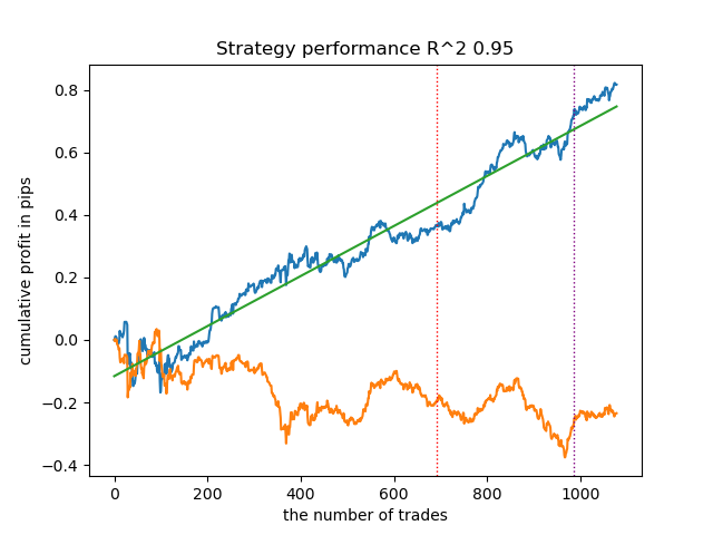
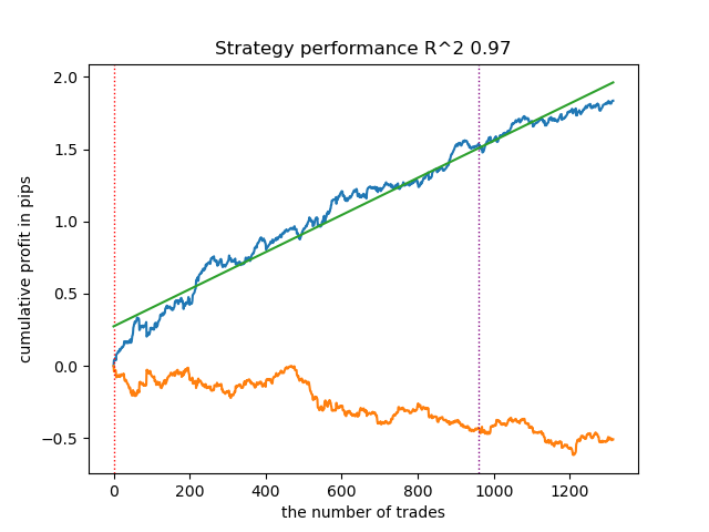
All proposed clustering algorithms were analyzed to determine market regimes. Some algorithms performed well, while others performed poorly.

Below are the training results using different clustering algorithms:

First of all, I was interested in the clustering speed. Affinity Propagation, Spectral Clustering, Agglomerative Clustering and Mean Shift algorithms were found to be very slow, which is why they are all at the bottom of the ranking. I was unable to obtain clustering results using standard settings, so results for these algorithms are not shown.

I found a confirmation to this on the web:

I ran 10 iterations of the entire training process for more informative results, because the results differ in different training iterations due to randomization within the algorithms.

• Blue line displays a balance graph.
• Orange line is the financial instrument chart (in this case EURUSD).

1. Among the four remaining algorithms, I decided to put HDBSCAN at the top of the rating. It separates the data well and does not require setting the number of clusters.

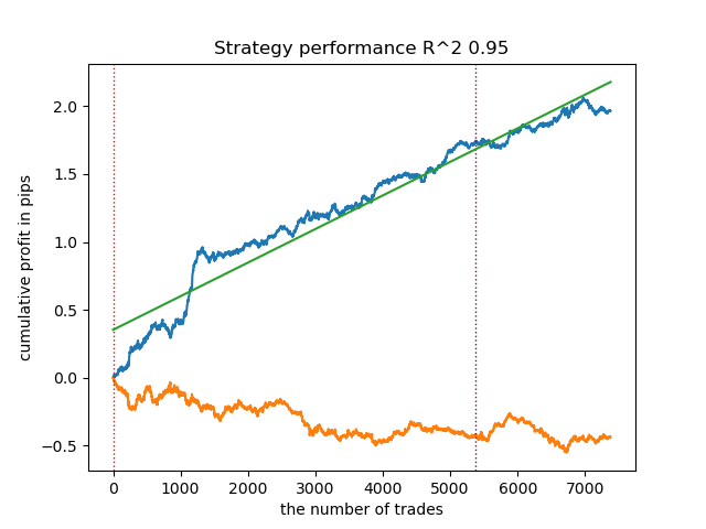
2. K-means shows good performance and quite good testing results. The downside is the sensitivity to the number of clusters, in this case it is ten.

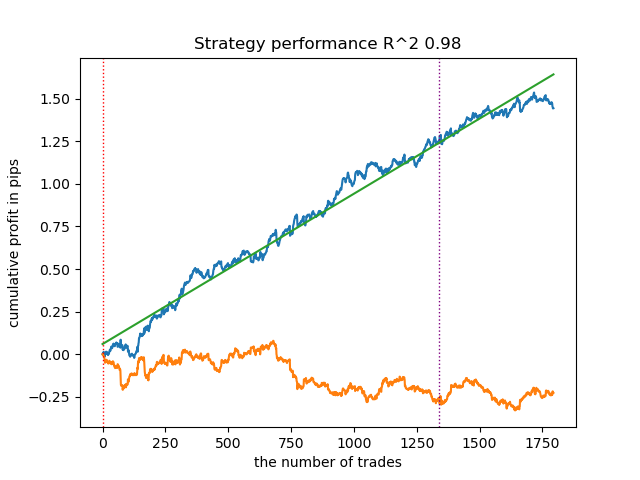
3. BIRCH shows good results, but it calculates somewhat slower than previous algorithms. There is also no requirement for an initial number of clusters.

4. Gaussian mixture completes this rating. The test results seemed worse to me than when using other clustering algorithms. Visually, this is expressed in a "noisier" balance graph. As with K-means, we defined 10 clusters.

Thus, we can get different trading systems, depending on the selected market regime. During the training process, model testing results are displayed each regime, based on a specified number of clusters.

The quality of clustering is affected by the set of input parameters. Below are the parameters we used:

• Currency Pair
• Time Frame
• Start and end dates of training
• Number of features for the main model
• Number of features for the meta model (volatility)
• Number of clusters n_clusters
• Parameters 'min' and 'max' of the get_labels(min, max) function

For example, here is another set of clustering results with the following parameters:

SYMBOL = 'EURUSD'
MARKUP = 0.00010
PERIODS = [i for i in range(10, 100, 10)]
PERIODS_META = [20]
BACKWARD = datetime(2019, 1, 1)
FORWARD = datetime(2023, 1, 1)
n_clusters = 40

def get_labels(dataset, min = 5, max = 5)

Timeframe = H1

Since the cluster search algorithm is also randomized, it is good practice to run it several times.

Matching trades using clustering

Let's move on to the final part, which is actually the main part of the article. I wanted to deepen the understanding of causal inference by adding a clustering element to it. This article explains causal inference is, and another article covers matching through Propensity Score. Now let's replace matching through the propensity score with our own approach, i.e., matching through clustering. For these purposes, we will use the algorithm from the first article and modify it.

def meta_learners(models_number: int, iterations: int, depth: int, bad_samples_fraction: float, n_clusters: int):
    dataset = get_labels(get_prices())
    data = dataset[(dataset.index < FORWARD) & (dataset.index > BACKWARD)].copy()

    X = data[data.columns[1:-2]]
    y = data['labels']
    clusters = KMeans(n_clusters=n_clusters).fit(X[X.columns[0:1]]).labels_

    BAD_CLUSTERS = []
    for _ in range(n_clusters):
        sublist =  [pd.DatetimeIndex([]), pd.DatetimeIndex([])]
        BAD_CLUSTERS.append(sublist)

    for i in range(models_number):
        X_train, X_val, y_train, y_val = train_test_split(
            X, y, train_size = 0.5, test_size = 0.5, shuffle = True)
        
        # learn debias model with train and validation subsets
        meta_m = CatBoostClassifier(iterations = iterations,
                                depth = depth,
                                custom_loss = ['Accuracy'],
                                eval_metric = 'Accuracy',
                                verbose = False,
                                use_best_model = True)
        
        meta_m.fit(X_train, y_train, eval_set = (X_val, y_val), plot = False)
        
        coreset = X.copy()
        coreset['labels'] = y
        coreset['labels_pred'] = meta_m.predict_proba(X)[:, 1]
        coreset['labels_pred'] = coreset['labels_pred'].apply(lambda x: 0 if x < 0.5 else 1)
        coreset['clusters'] = clusters
        
        # add bad samples of this iteration (bad labels indices)
        coreset_b = coreset[coreset['labels']==0]
        coreset_s = coreset[coreset['labels']==1]

        for clust in range(n_clusters):
            diff_negatives_b = (coreset_b['labels'] != coreset_b['labels_pred']) & (coreset['clusters'] == clust)
            diff_negatives_s = (coreset_s['labels'] != coreset_s['labels_pred']) & (coreset['clusters'] == clust)
            BAD_CLUSTERS[clust][0] = BAD_CLUSTERS[clust][0].append(diff_negatives_b[diff_negatives_b == True].index)
            BAD_CLUSTERS[clust][1] = BAD_CLUSTERS[clust][
        1].append(diff_negatives_s[diff_negatives_s == True].index)

    for clust in range(n_clusters):
        to_mark_b = BAD_CLUSTERS[clust][0].value_counts()
        to_mark_s = BAD_CLUSTERS[clust][1].value_counts()
        marked_idx_b = to_mark_b[to_mark_b > to_mark_b.mean() * bad_samples_fraction].index
        marked_idx_s = to_mark_s[to_mark_s > to_mark_s.mean() * bad_samples_fraction].index
        data.loc[data.index.isin(marked_idx_b), 'meta_labels'] = 0.0
        data.loc[data.index.isin(marked_idx_s), 'meta_labels'] = 0.0

    return data[data.columns[1:]]

For those who have not read my previous articles, I will give a brief description of the algorithm:

• Data processing:
• At the beginning, we use the get_prices() and get_labels() functions to get the dataset. These functions return price information and class labels, respectively.
• get_labels() associates price data with labels, which is a common task in ML related to financial data.
• The data is then filtered by time intervals defined by FORWARD and BACKWARD constants.
• Data preparation:
• The data is divided into features (X) and labels (y).
• Then we use the KMeans clustering algorithm to create data clusters.
• Model training:
• In a for loop, we determine the number of models is models_number. In each iteration, the model is trained on half of the dataset (train_size = 0.5) and validated on the second half (validation set).
• We use the CatBoostClassifier model with certain parameters. This gradient boosting method is specifically designed to work with categorical features.
• Please note that the algorithm uses the custom loss function 'Accuracy' and the evaluation metric 'Accuracy'. This indicates that we focus on prediction accuracy.
• The meta-model is then applied to evaluate and adjust the predictions of the primary models. This allows us to take into account possible biases or errors in the primary models.
• Identifying bad samples:
• The algorithm creates BAD_CLUSTERS lists containing which information about the bad samples in each cluster. Bad samples are defined as those for which the model makes a significant number of errors.
• For each training iteration, the algorithm identifies bad samples and saves their indexes in the corresponding list.
• Meta-analysis and correction:
• The indexes of the bad samples identified in the previous step are aggregated and then used to flag the corresponding samples in the master data.
• This is supposed to help improve the quality of model training by eliminating or correcting bad samples.
• Return data:
• The function returns the prepared data without the first column, which contains timestamps.

This algorithm strives to improve the quality of machine learning models by detecting and correcting bad samples, and using a meta-model to account for errors in the primary models. It is complex and requires careful tuning of parameters to work effectively.

In the presented code, clustering helps to account for heterogeneity in the data in several ways:

• Identifying data clusters:
• Using the KMeans clustering algorithm allows us to divide data into groups of similar objects. Each cluster contains data with similar characteristics. This is especially useful in the case of heterogeneous data, where objects may belong to different categories or have different structures.
• Analysis and processing of clusters separately:
• Each cluster is processed separately from the others, which makes it possible to take into account data characteristics and structure within each group. This assist in understanding the heterogeneity of data and adapting learning algorithms to specific conditions in each cluster.
• Error correction within clusters:
• After training the models, bad samples for each cluster are analyzed in a loop. These are the samples for which the model makes a significant number of errors. This allows you to localize and focus error correction within each cluster separately, which can be more effective than applying the same corrections to all data as a whole.
• Taking into account data features in meta-model training:
• Clustering is also used to account for differences between clusters when training a meta-model. This allows the meta-model to better adapt to data heterogeneity by incorporating information about the structure of the data within each cluster.

Thus, clustering plays a key role in accounting for data heterogeneity, allowing the algorithm to more effectively adapt to the diversity of objects and data structures.

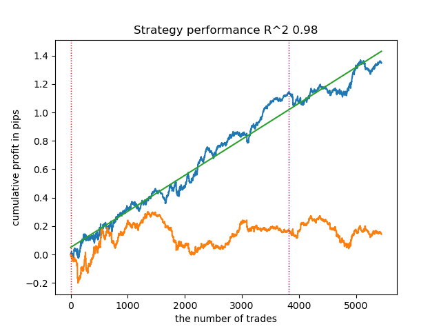
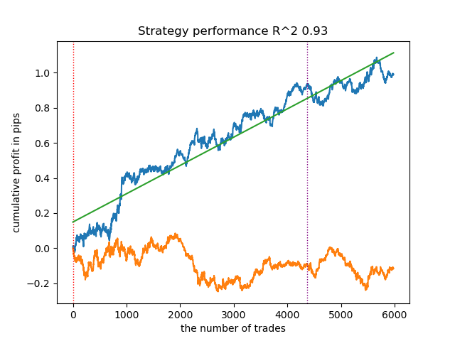
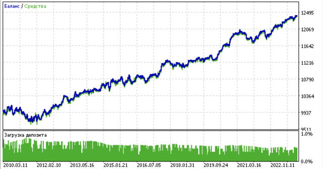
The model training results are shown below. You can see that the model has become more stable with new data.

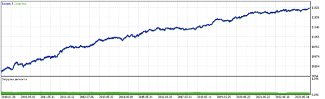
This model can be exported to ONNX format and is fully compatible with the ONNX Trader EA.

Conclusion

In this article, we discussed the author's original approach to time series clustering. I tested various algorithms for clustering market regimes by volatility. I found that complex algorithms do not always live up to expectations: sometimes simple and fast clustering algorithms like K-means do a better job. At the same time, I really liked the HDBSCAN algorithm.

In the second part, clustering was used to determine the heterogeneous treatment effect. Experiments have shown that taking into account bad trades using clustering reduces the range of values (the balance curve becomes smoother) and improves the model's capability to predict on new data. In general, this is a rather complex and deep topic that requires configuration of hyperparameters to fine-tune the algorithm.