Propensity score in causal inference

Introduction

We continue our immersion into the world of causal inference and its modern tools. Of course, the task is somewhat broader - the use of causal inference methods in trading. We have already started by studying the basics and even wrote our first meta learners, which, by the way, turned out to be quite robust. Or rather, the models that were obtained with their help turned out to be robust. It is worth mentioning that they were the first ones only for the reader, since they are just another experiment for the writer. Therefore, there is no turning back and we will have to go to the end until the whole topic of causal inference in trading is covered. After all, approaches to causal inference can be different, and I would like to cover this interesting topic as widely as possible.

In this article, I will cover the topic of matching briefly mentioned in the previous article, or rather one of its varieties - propensity score matching. 

This is important because we have a certain set of labeled data that is heterogeneous. For example, in Forex, each individual training example may belong to the area of high or low volatility. Moreover, some examples may appear more often in the sample, while some appear less often. When attempting to determine the average causal effect (ATE) in such a sample, we will inevitably encounter biased estimates if we assume that all examples in the sample have the same propensity to produce treatment. When trying to obtain a conditional average treatment effect (CATE), we may encounter a problem called the "curse of dimensionality".

Matching is a family of methods for estimating causal effects by matching similar observations (or units) in treatment and control groups. The purpose of matching is to make comparisons between similar units to achieve as accurate an estimate of the true causal effect as possible.

Some authors of the causal inference literature suggest that matching should be considered a data preprocessing step on top of which any estimator (e.g., meta learner) can be used. If we have enough data to potentially discard some observations, using matching as a preprocessing step is usually useful. 

Imagine you have a data set to analyze. This data contains 1000 observations. What are the chances that you will find at least one exact match for each row if you have 18 variables in your data set? The answer obviously depends on a number of factors. How many variables are binary? How many of them are continuous? How many of them are categorical? How many levels do categorical variables have? Are the variables independent or correlated with each other?

Aleksander Molak gives a good visual example in his book "Causal inference and discovery in Python".

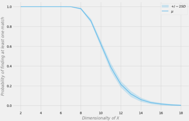
Probability of finding an exact match depending on the dimension of the data set

Let's assume that our sample has 1000 observations. In the figure above, the X axis represents the dimension of the data set (the number of variables in the data set), and the Y axis represents the probability of finding at least one exact match in each row.

The blue line is the average probability and the shaded areas represent +/- two standard deviations. The data set was generated using independent Bernoulli distributions with p = 0.5. Therefore, each variable is binary and independent. 

I decided to test this statement from the book and wrote a Python script that calculates this probability.

import numpy as np
import matplotlib.pyplot as plt

def calculate_exact_match_probability(dimensions):
    num_samples = 1000
    num_trials = 1000
    match_count = 0

    for _ in range(num_trials):
        dataset = np.random.randint(2, size=(num_samples, dimensions))
        row_sums = np.sum(dataset, axis=1)
        if any(row_sums == dimensions):
            match_count += 1

    return match_count / num_trials

def plot_probability_curve(max_dimensions):
    dimensions_range = list(range(1, max_dimensions + 1))
    probabilities = [calculate_exact_match_probability(dim) for dim in dimensions_range]

    mean_probability = np.mean(probabilities)
    std_dev = np.std(probabilities)

    plt.plot(dimensions_range, probabilities, label='Exact Match Probability')
    plt.axhline(mean_probability, color='blue', linestyle='--', label='Mean Probability')

    plt.xlabel('Number of Variables')
    plt.ylabel('Probability')
    plt.title('Exact Match Probability in Binary Dataset')
    plt.legend()
    plt.show()

Indeed, for 1000 observations the probabilities coincided. As an experiment, you can calculate them for the dimensions of your datasets yourself. For our further work, it is enough to understand that if there are too many features (covariates) in the data compared to the number of training examples, then the ability to generalize such data through the classifier will be limited. The greater the amount of data, the more accurate the statistical estimates.

*In real practice, this is not always the case, since the i.i.d ((independent and identically-distributed)) condition should be met.

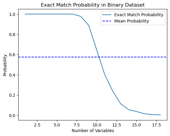
As you can see, the probability of finding an exact match in an 18-dimensional binary random data set is essentially zero. In real world, we rarely work with purely binary data sets, and for continuous data, multidimensional mapping becomes even more difficult. This poses a serious problem for matching, even in the approximate case. How can we solve this issue?

Reducing data dimensionality using propensity score

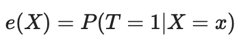
We can solve the curse of dimensionality problem using the propensity score. Propensity scores are estimates of the probability that a given unit will be assigned to the experimental group based on its characteristics. According to the propensity score theorem (Rosenbaum and Rubin, 1983), if we have unconfounded data for X trait, we will also have unconfoundedness given the propensity score, while assuming positivity. Positivity means that treated and untreated distributions should overlap. This is the causal inference positivity assumption. This also makes intuitive sense. If the test group and control group do not overlap, this means that they are very different and we cannot extrapolate the effect of one group to the other. This extrapolation is not impossible (regression makes it), but it is very dangerous. This is similar to testing a new medicine in an experiment where only men are given the treatment, and then assuming that women will respond equally well to it.

Formally, the propensity score is written as follows:

In a perfect world, we would have a true propensity score. However, in practice, the mechanism for assigning treatment is unknown, and we need to replace the true predisposition with its assessment or expectation. One common way to do this is to use logistic regression, but other machine learning techniques such as gradient boosting can be used (although this requires some additional steps to avoid overfitting).

We can use this equation to solve the problem of multidimensionality. Propensity scores are univariate, and so we can now only match two values rather than multivariate vectors.

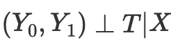
Thus, if we have the conditional independence of potential outcomes from treatment,

then we can calculate the average causal effect for continuous and discrete cases when matching without propensity score:

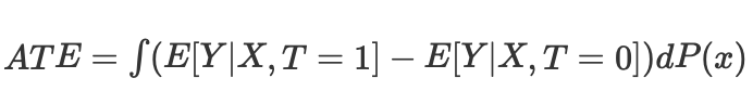
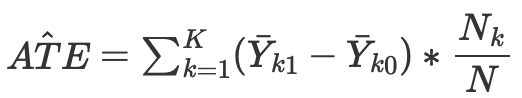
where Nk is the number of observations in each cell. A cell is a subgroup of observations matched by some proximity metric.

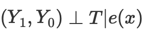
However, the propensity score arises from the realization that we do not need to directly control X confounding factors to achieve conditional independence

Instead, it is enough to control the balancing indicator

The propensity score allows one to be independent of X as a whole to ensure that potential outcomes are independent of treatment. It is sufficient to condition on this single variable, which is a propensity score:

The sources on causal inference describes a number of issues with this approach:

• First, propensity scores reduce the dimensionality of our data and, by definition, force us to throw out some information.

• Second, two observations that are very different in the original feature space may have the same propensity score. This can lead to very different observations matching and therefore biasing the results.

• Thirdly, PSM (Propensity score modeling) leads to a paradox. In the binary case, the optimal propensity score would be 0.5. What happens in a perfect scenario where all observations have an optimal propensity score of 0.5? The position of each observation in propensity score space becomes identical to every other observation. This is sometimes called the PSM paradox. 

Propensity score matching and related methods

There are a number of methods for matching units based on propensity score. The main method is considered to be the nearest neighbors method, which matches each unit i in the experimental group with unit j in the control group with the nearest absolute distance between their propensity scores, expressed as

d(i, j) = minj{|e(Xi) – e(Xj)|}.

Alternatively, threshold matching matches each unit i in the treatment group with unit j in the control group within a prespecified b; threshold that is

d(i, j) = minj{|e(Xi) – e(Xj)| <b}.

It is recommended that the b prespecified threshold be less than or equal to 0.25 standard deviations of the propensity scores. Other researchers argue that b = 0.20 of the propensity scores standard deviation is optimal. 

Another option of threshold matching is radius matching, which is a one-to-many matching and matches each unit i in the treatment group with several units in the control group within the b predefined range; that is

d(i, j) = {|e(Xi) – e(Xj)| <b}.

Other propensity score matching methods include the Mahalanobis metric. In matching using the Mahalanobis metric, each unit i in the experimental group is matched with unit j in the control group, with the nearest Mahalanobis distance calculated based on the proximity of the variables.

The propensity score matching methods discussed so far can be implemented using either a greedy matching algorithm or an optimal matching algorithm.

• In greedy matching, once the matching is done, the matched units cannot be changed. Each pair of matched units is the best pair currently available. 

• With optimal matching, previous matched units can be modified before performing the current matching to achieve an overall minimum or optimal distance. 

• Both matching algorithms typically produce the same matching data when the control group size is large. However, optimal matching results in smaller overall distances within matched units. Thus, if the goal is simply to find well-matched groups, greedy matching may be sufficient. If the goal is instead to find well-matched pairs, then optimal matching may be preferable.

There are methods associated with propensity score matching that do not strictly match individual sampling units. For example, subclassification (or stratification) classifies all units in the entire sample into several strata based on the corresponding number of propensity score percentiles and matches the units by stratum. Five strata have been observed to eliminate up to 90% of selection bias.

A special type of subclassification is full matching, in which subclasses are created in an optimal way. A fully matched sample consists of matched subsets, in which each matched set contains one experimental unit and one or more control units, or one control unit and one or more experimental units. Full matching is optimal in terms of minimizing the weighted average of the estimated distance measure between each treatment subject and each control subject in each subclass.

Another method associated with propensity score matching is kernel matching (or local linear matching), which combines matching and outcome analysis in a single procedure with one-to-all matching.

Despite the variety of proposed comparison methods, the efficiency of their application depends more on the correct formulation of the problem than on a specific method.

Strong neglect assumption

"Strong neglect" is a crucial assumption in the construction of the propensity score, which aims to estimate causal effects in observations where treatment assignment is random. Essentially, this means that treatment assignment is independent of potential outcomes given observed baseline covariates (traits). 

Let's take a closer look:

• Treatment distribution: This is whether a unit receives treatment or not (such as taking a new medication or participating in a program).

• Potential outcomes: These are the outcomes that a unit would experience in both the treatment and control conditions, but we can only observe one for each unit.

• Baseline covariates: These are unit characteristics measured before treatment allocation that may influence both the likelihood of receiving treatment and the outcome.

The "strongly ignorable" assumption states that:

• No unmeasured confounders: There are no unobserved variables that influence either treatment allocation or outcome. This is important because unobserved confounders may bias the estimated treatment effect.

• Positivity: Each unit has a nonzero probability of receiving both treatment and control, given its observed covariates. This ensures that there are enough units in the groups being compared to make meaningful comparisons.

If these conditions are met, then conditioning on the propensity score (the estimated probability of receiving treatment given covariates) produces unbiased estimates of the average treatment effect (ATE). ATE represents the mean difference in outcomes between treatment and control groups as if treatment had been randomly assigned.

Inverse probability weighting

Inverse probability weighting is one of the approaches implying eliminating noise or confounding factors by attempting to re-weight observations in a data set based on the inverse of the probability of treatment assignment. The idea is to give more weight to observations that are rated as less likely to be treated by treatment, making them more representative of the general population.

• First, a propensity score is estimated, which is the probability of receiving treatment given the observed covariates.

• An inverse propensity score is calculated for each observation.

• Each observation is then multiplied by its corresponding weight. This means that observations with a lower probability of receiving the observed treatment are given more weight.

• The weighted data set is then used for analysis. Weights are applied to both the treatment and control groups, adjusting for the potential influence of observed covariates.

Inverse probability weighting can help balance the distribution of covariates between treatment and control groups, reducing bias in estimating causal effects. However, it is based on the assumption that all relevant confounding variables are measured and included in the model used to estimate the propensity score. Additionally, like any statistical method, the success of IPW depends on the quality of the model used to estimate the propensity score.

The inverse propensity score equation is as follows:

Without going into detail, you can compare the two terms of the equation. The left one is for the treatment group, while the right one is for the control group. The equation shows that a simple comparison of averages is equivalent to a comparison of inversely weighted averages. This creates a population the same size as the original, but in which everyone on the left side receives the treatment. For the same reasons, the right one considers untreated ones and puts a high value on those that look like treated ones.

Evaluation of results after matching

In causal inference, the estimate is constructed as ATE or CATE, that is, the difference in the weighted means (adjusted for the propensity score) of the treated and untreated target values. 

Once we have obtained the propensity score as e(x), we can use these values, for example, to train another classifier, instead of the original values of X features. We can also compare samples by their propensity score to divide them into strata. Another option is to add e(x) as a separate feature when training the final evaluator, which will help eliminate biased estimates due to confounding, when different examples in the sample have different estimates according to propensity score.

We are interested in finding subgroups that respond well or poorly to treatment (model training) and then train the final classifier only on data that can be trained well (the classification error is minimal). Then we should put the poorly classified data into the second subgroup and train the second classifier to distinguish between these two subgroups, that is, to separate the wheat from the chaff, or to identify subgroups that are most amenable to treatment. Therefore, we will not now adopt the entire propensity score methodology, but will match the samples according to the obtained probabilities of the trained classifier, while the overall ATE (average treatment effect) assessment is of little interest to us.

In other words, we will base our assessment on the results of the algorithm running on new data that did not participate in training. Additionally, we are still interested in the average speed of a set of models trained on randomized data. The higher the average score of independent models, the more confidence we have in each specific model.

Moving on to experiments

When starting this article, I was aware that for many traders, especially those unfamiliar with machine learning, this in-depth material may seem very counterintuitive. Remembering my first encounter with causal inference, this initial misunderstanding hurt my pride so much that I simply could not help but delve into the details. Moreover, I could not even imagine that I would take the liberty of adapting causal inference techniques to classify time series.

• propensity without matching.py file

Let's start with a way we can incorporate propensity scores directly into our estimator, or meta learner. To do this, we need to train two models. First, the PSM (propensity score model) itself, which will allow us to obtain the probabilities of assigning training examples to treatment or test groups. We will feed the obtained probabilities, together with the characteristics (covariates), as input to the second model, which will predict the outcomes (buy or sell).

The intuition of this approach is that the meta learner will now be able to distinguish subgroups of samples based on their tendency to treat. This will give us weighted predictions of outcomes that should be more accurate. After this, we will divide the dataset into well-predictable and poorly predictable cases, as was the case in previous articles. In this case, we will not need explicit sample matching because the meta learner will automatically take the propensity score into account in its estimates. This approach seems quite convenient to me, because machine learning does all the work for us.

First, let's create 'train' and 'val' subsamples to train the meta model. Since the meta learner will be trained on the train subsample, we will create a pair of target y_T1, y_T0, and fill them with ones and zeros. This will correspond to whether the units received treatment (model training) or not. Then we re-shuffle the subselection whose target variables are treatments.

        X_train, X_val, y_train, y_val = train_test_split(
            X, y, train_size = 0.5, test_size = 0.5, shuffle = True)
        
        # randomly assign treated and control
        y_T1 = pd.DataFrame(y_train)
        y_T1['T'] = 1
        y_T1 = y_T1.drop(['labels'], axis=1)

        y_T0 = pd.DataFrame(y_val)
        y_T0['T'] = 0
        y_T0 = y_T0.drop(['labels'], axis=1)

        y_TT = pd.concat([y_T1, y_T0])
        y_TT = y_TT.sort_index()

        X_trainT, X_valT, y_trainT, y_valT = train_test_split(
            X, y_TT, train_size = 0.5, test_size = 0.5, shuffle = True)

The next step is to train the PSM model to predict whether samples belong to the treatment or control subsamples.

        # fit propensity model
        PSM = CatBoostClassifier(iterations = iterations,
                                depth = depth,
                                custom_loss = ['Accuracy'],
                                eval_metric = 'Accuracy',
                                use_best_model=True,
                                early_stopping_rounds=15,
                                verbose = False).fit(X_trainT, y_trainT, eval_set = (X_valT, y_valT), plot = False)

Then we need to get predictions of belonging to the treatment and control groups and add them to the characteristics of the meta learner, and then train it.

        # predict probabilities
        train_proba = PSM.predict_proba(X_train)[:, 1]
        val_proba = PSM.predict_proba(X_val)[:, 1]

        # fit meta-learner
        meta_m = CatBoostClassifier(iterations = iterations,
                                depth = depth,
                                custom_loss = ['Accuracy'],
                                eval_metric = 'Accuracy',
                                verbose = False,
                                use_best_model = True,
                                early_stopping_rounds=15).fit(X_train.assign(T=train_proba), y_train, 
				eval_set = (X_val.assign(T=val_proba), y_val), plot = False)
        

At the final stage, we will obtain the meta learner predictions, compare the predicted labels with the actual ones, and fill out the book of bad examples.

        # create daatset with predicted values
        predicted_PSM = PSM.predict_proba(X)[:,1]
        X_psm = X.assign(T=predicted_PSM)
        coreset = X.assign(T=predicted_PSM)
        coreset['labels'] = y
        coreset['labels_pred'] = meta_m.predict_proba(X_psm)[:,1]
        coreset['labels_pred'] = coreset['labels_pred'].apply(lambda x: 0 if x < 0.5 else 1)

        # add bad samples of this iteration (bad labels indices)
        coreset_b = coreset[coreset['labels']==0]
        coreset_s = coreset[coreset['labels']==1]

        diff_negatives_b = coreset_b['labels'] != coreset_b['labels_pred']
        diff_negatives_s = coreset_s['labels'] != coreset_s['labels_pred']
        BAD_BUY = BAD_BUY.append(diff_negatives_b[diff_negatives_b == True].index)
        BAD_SELL = BAD_SELL.append(diff_negatives_s[diff_negatives_s == True].index)

Now let's try to train 25 models and look at the best and average results.

options = []
best_res = 0.0
for i in range(25):
    print('Learn ' + str(i) + ' model')
    options.append(learn_final_models(meta_learners(models_number=5, 
                                                    iterations=25, 
                                                    depth=2,
                                                    bad_samples_fraction=0.5)))
    if options[-1][0] > best_res:
        best_res = options[-1][0]
    print("BEST: " + str(best_res))

options.sort(key=lambda x: x[0])
test_model(options[-1][1:], plt=True)
test_all_models(options)

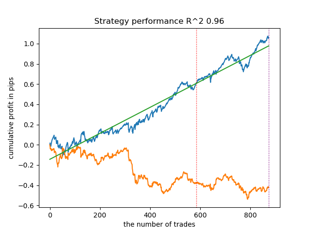
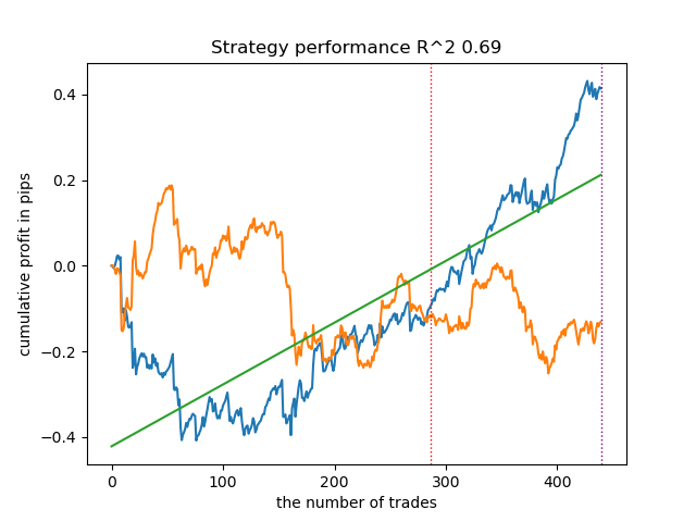
I conducted a series of such trainings and concluded that this approach is practically no different in the quality of models from my approach described in the previous article. Both options are capable of generating good models that pass OOS. This should not surprise us, because we used e(x) as an additional feature, and the rest of the algorithm remained unchanged.

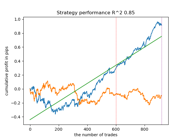
• propensity matching naive.py file

When considering implementation methods, we can never know in advance, which method will work better. As an experiment, I decided to do a match not by the propensity to assign treatment, but by the propensity to predict target labels. This should seem more intuitive to the reader. The main difference here is that we train only one (conventionally named) PSM model. Next, the probabilities are predicted and a list of bins is created according to the number of strata into which we want to divide the obtained probabilities. For each stratum, the number of correctly/incorrectly guessed outcomes is counted, after which for strata where the number of incorrectly guessed (multiplied by a ratio) examples exceeds the number of correctly guessed ones, the condition for adding bad examples to the book of bad examples is triggered.

        bins = np.linspace(lower_bound, upper_bound, num=bins_number)
        coreset['bin'] = pd.cut(coreset['propensity'], bins)
        

        for val in range(len(coreset['bin'].unique())):
            values = coreset.loc[coreset['bin'] == coreset['bin'].unique()[val]]
            diff_negatives = values['labels'] != values['labels_pred']
            if len(diff_negatives[diff_negatives == False]) < (len(diff_negatives[diff_negatives == True]) * coefficient):
                B_S_B = B_S_B.append(diff_negatives[diff_negatives == True].index)

This approach has additional parameters:

• bins_number - number of bins
• lower_bound - lower probability limit strata are calculated from
• upper_bound - upper probability limit, up to which strata are calculated

Since we are using a meta learner with little depth, the probabilities usually cluster around 0.5 and rarely reach extreme limits. Therefore, we can discard extreme values as uninformative by setting upper and lower bounds.

Let's train 25 models and look at the results. I would like to note that all models are trained on the same dataset, so their comparison is quite correct.

options = []
best_res = 0.0
for i in range(25):
    print('Learn ' + str(i) + ' model')
    options.append(learn_final_models(meta_learners(models_number=5, 
                                                    iterations=25, 
                                                    depth=2,
                                                    bad_samples_fraction=0.5,
                                                    bins_number=25,
                                                    lower_bound=0.3,
                                                    upper_bound=0.7,
                                                    coefficient=1.0)))
    if options[-1][0] > best_res:
        best_res = options[-1][0]
    print("BEST: " + str(best_res))

options.sort(key=lambda x: x[0])
test_model(options[-1][1:], plt=True)

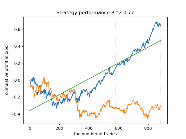
Surprisingly, this spontaneous implementation performed quite well on the new data. Below are trading charts for the best model and all 25 models at once.

• propensity matching original.py file

We proceed to the implementation of the example closest to the theory, in which the assumption of strong neglect (strongly ignorable) is fulfilled. Let me remind you that "strongly ignorable" is when the assignment of treatment does not depend in any way on potential outcomes, which means it is completely random and there are no unaccounted variables that influence bias. To do this, we will randomly assign a treatment and train the PSM model. Then we train the meta estimator to predict the outcomes of trades (class labels). After this, we stratify the sample according to the propensity score and add samples to the book of bad examples only from those bins, in which the number of unsuccessful predictions exceeds the number of successful ones, taking into account the ratio.

I also added the ability to use IPW (inverse probability weighting) described in the theoretical part.

After training two classifiers, the following code is executed.

        # create daatset with predicted values
        coreset = X.copy()
        coreset['labels'] = y
        coreset['propensity'] = PSM.predict_proba(X)[:, 1]
        if Use_IPW:
            coreset['propensity'] = coreset['propensity'].apply(lambda x: 1 / x if x > 0.5 else 1 / (1 - x))

        coreset['propensity'] = coreset['propensity'].round(3)
        coreset['labels_pred'] = meta_m.predict_proba(X)[:, 1]
        coreset['labels_pred'] = coreset['labels_pred'].apply(lambda x: 0 if x < 0.5 else 1)

        bins = np.linspace(lower_bound, upper_bound, num=bins_number)
        coreset['bin'] = pd.cut(coreset['propensity'], bins)        

        for val in range(len(coreset['bin'].unique())):
            values = coreset.loc[coreset['bin'] == coreset['bin'].unique()[val]]
            diff_negatives = values['labels'] != values['labels_pred']
            if len(diff_negatives[diff_negatives == False]) < (len(diff_negatives[diff_negatives == True]) * coefficient):
                B_S_B = B_S_B.append(diff_negatives[diff_negatives == True].index)

Let's train 25 models without using IPW and look at the best balance graph and the one averaged over all models, with the following settings:

options = []
best_res = 0.0
for i in range(25):
    print('Learn ' + str(i) + ' model')
    options.append(learn_final_models(meta_learners(models_number=5, 
                                                    iterations=25, 
                                                    depth=2,
                                                    bad_samples_fraction=0.5,
                                                    bins_number=25,
                                                    lower_bound=0.3,
                                                    upper_bound=0.7,
                                                    coefficient=1.5,
                                                    Use_IPW=False)))
    if options[-1][0] > best_res:
        best_res = options[-1][0]
    print("BEST: " + str(best_res))

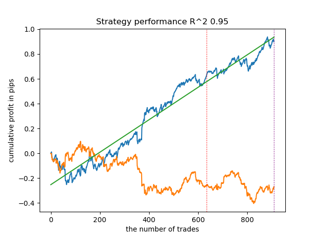
In general, the results are comparable to the results of previous implementations. Now let's do the same with IPW enabled.

options = []
best_res = 0.0
for i in range(25):
    print('Learn ' + str(i) + ' model')
    options.append(learn_final_models(meta_learners(models_number=5, 
                                                    iterations=25, 
                                                    depth=2,
                                                    bad_samples_fraction=0.5,
                                                    bins_number=25,
                                                    lower_bound=0.1,
                                                    upper_bound=10.0,
                                                    coefficient=1.5,
                                                    Use_IPW=True)))
    if options[-1][0] > best_res:
        best_res = options[-1][0]
    print("BEST: " + str(best_res))

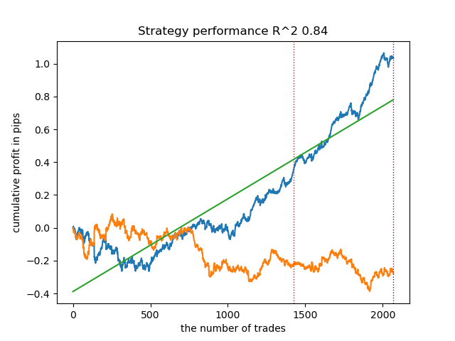
The results turned out to be some of the best. Of course, for a more detailed comparison, it is necessary to carry out multiple tests on different symbols, but this would increase the volume of an already large article. The table of the results obtained is presented below.

Algorithm	Best result	Average result (25 models)
propensity without matching.py	0.96	0.69
propensity matching naive.py	0.94	0.85
propensity matching original.py	0.95	0.77
propensity matching original.py IPW	0.97	0.84

Conclusion

We considered the possibility of using the propensity score for the problem of classifying financial time series. This approach has good theoretical justification in the area of causal inference, but it also has its shortcomings. In general, it allowed us to obtain models that retain their characteristics on new data.