MQL5 Wizard Techniques you should know (Part 33): Gaussian Process Kernels

Introduction

Gaussian Process Kernels are covariance functions used in Gaussian processes to measure the relationships among data points, such as in a time series. These kernels generate matrices that capture the intra-data relationship, allowing the Gaussian Process to make projections or forecasts by assuming the data follows a normal distribution. As these series look to explore new ideas while also examining how these ideas can be exploited, Gaussian Process (GP) Kernels are serving as our subject in building a custom signal.

We have recently covered a lot of machine learning related articles over the past five articles, so for this one we ‘take a break’ and look at good old statistics. In the nature of developing systems quite often the two are married, however in developing this particular custom signal we will not be supplementing or considering any machine learning algorithms. GP kernels are noteworthy because of their flexibility.

They can be used to model a wide variety of data patterns that range in focus from periodicity, to trends or even non-linear relationships. However, more significant than this is when predicting, they do more than provide a single value. Instead, they provide an uncertainty estimate that would include the desired value, as well as an upper bound and lower bound value. These bound ranges are often provided with a confidence rating, which further facilitates a trader’s decision-making process when presented with a forecast value. These confidence ratings can also be insightful and help in better understanding traded securities when comparing different forecast bands that are marked with disparate confidence levels.

In addition, they are good at handling noisy data since they allow a noise value to be incremented to the created K matrix (see below), and they also are capable of being used while incorporating prior knowledge into them, plus they are very scalable. There are quite a number of different kernels to choose from out there. The list includes (but is not limited to): Squared Exponential Kernel (RBF), Linear kernel, Periodic kernel, Rational quadratic kernel, Matern kernel, Exponential kernel, Polynomial kernel, White noise kernel, Dot product kernel, Spectral mixture kernel, Constant kernel, Cosine kernel, Neural network (Arccosine) kernel, and Product & Sum kernels.

For this article we are just going to look at the RBF kernel aka Radial Basis Function kernel. Like most kernels, it measures similarity between any two data points by focusing on their distance apart with an underlying basic assumption that the further points are the less similar they are and vice versa. This is governed by the following equation:

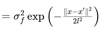
Where

• x and x′:These are the input vectors or points in the input space.
• σ f ²:This is the variance parameter of the kernel, which serves as a pre-determined or optimizable parameter.
• l is often referred to as the length-scale parameter. It controls the smoothness of the resulting function. A smaller l (or shorter length scale) results in a rapidly varying function, while a larger l (longer length scale) results in a smoother function.
• exp: This is the exponential function.

This kernel can be coded in MQL5 easily as:

//+------------------------------------------------------------------+
// RBF Kernel Function
//+------------------------------------------------------------------+
matrix CSignalGauss::RBF_Kernel(vector &Rows, vector &Cols)
{  matrix _rbf;
   _rbf.Init(Rows.Size(), Cols.Size());
   for(int i = 0; i < int(Rows.Size()); i++)
   {  for(int ii = 0; ii < int(Cols.Size()); ii++)
      {  _rbf[i][ii] = m_variance * exp(-0.5 * pow(Rows[i] - Cols[ii], 2.0) / pow(m_next, 2.0));
      }
   }
   return(_rbf);
}

Gaussian Processes within Financial Time Series

Gaussian processes are a probabilistic framework where forecasts are made in terms of distributions rather than fixed values. This is why it’s also referred to as a non-parametrized framework. The output forecasts include a mean prediction and a variance (or uncertainty) around this forecast. The variance of GPs represents the uncertainty or confidence in the forecast made. This uncertainty is in principle random, given that it is based on the GP’s normal distribution. However, because it implies an interval and a confidence rating (usually based on 95%), not all its predictions need to be adhered to. Compared with other statistical forecasting methods like ARIMA, GP is highly flexible and capable of modelling complex non-linear relationships with uncertainty quantified, while ARIMA works best with stationary time series with set structures. The main downside to GP is it is computationally expensive, while methods like ARIMA are not.

The RBF Kernel

Computing the GP kernel involves principally 6 matrices and 2 vectors. These matrices and vectors are all used in our ‘GetOutput’ function, whose code is summarily given below:

//+------------------------------------------------------------------+
//|                                                                  |
//+------------------------------------------------------------------+
void CSignalGauss::GetOutput(double BasisMean, vector &Output)
{  
   ...

   matrix _k = RBF_Kernel(_past_time, _past_time);
   matrix _noise;
   _noise.Init(_k.Rows(), _k.Cols());
   _noise.Fill(fabs(0.05 * _k.Min()));
   _k += _noise;
   matrix _norm;
   _norm.Init(_k.Rows(), _k.Cols());
   _norm.Identity();
   _norm *= 0.0005;
   _k += _norm;
   vector _next_time;
   _next_time.Init(m_next);
   for(int i = 0; i < m_next; i++)
   {  _next_time[i] = _past_time[_past_time.Size() - 1] + i + 1;
   }
   matrix _k_s = RBF_Kernel(_next_time, _past_time);
   matrix _k_ss = RBF_Kernel(_next_time, _next_time);
// Compute K^-1 * y
   matrix _k_inv = _k.Inv();
   if(_k_inv.Rows() > 0 && _k_inv.Cols() > 0)
   {  vector _alpha = _k_inv.MatMul(_past);
      // Compute mean predictions: mu_* = K_s * alpha
      vector _mu_star = _k_s.MatMul(_alpha);
      vector _mean;
      _mean.Init(_mu_star.Size());
      _mean.Fill(BasisMean);
      _mu_star += _mean;
   // Compute covariance: Sigma_* = K_ss - K_s * K_inv * K_s^T
      matrix _v = _k_s.MatMul(_k_inv);
      matrix _sigma_star = _k_ss - (_v.MatMul(_k_s.Transpose()));
      vector _variances = _sigma_star.Diag();
      //Print(" sigma star: ",_sigma_star);
      Print(" pre variances: ",_variances);
      Output = _mu_star;
      SetOutput(Output);
      SetOutput(_variances);
      Print(" variances: ",_variances);
   }
}

To itemize these, they are:

• _k
• _k_s
• _k_ss
• _k_inv
• _v
• and_sigma_star

_k is the anchor and main covariance matrix. It captures the relationships across the pair of input vectors to the kernel function in use. We are using the Radial Basis Function (RBF) kernel, and its source has already been shared above. Since we are doing a forecast for a time series, the input to our RBF kernel would be two similar time vectors that log the time indices of the data series we are looking to forecast. By encoding similarities between logged time points, that serves as a basis for determining the overall structure. Keep in mind there are a lot of other kernel formats as is seen from the fourteen listed above and in future articles we could consider these alternatives as a custom signal class.

This leads us to the covariance matrix _k_s.This matrix acts as a bridge to the next time indices also via an RBF kernel like the_k matrix. The length or number of these time indices sets the number of projections to be made, and it's defined by the input parameter length-scale. We refer to this parameter as m_next in the custom signal class. By bridging pastime indices and the next time indices_k_sserves to project a relationship between known data and the next unknown data and this, as one would expect, is useful in the forecasting. This particular matrix is highly sensitive to the projection made, so its accuracy needs to be spot on, and gladly our code and RBF kernel function handle this seamlessly. Nonetheless, the two adjustable parameters of variance and length-scale need to be fine-tuned with care to ensure the accuracy of the projection is maximized.

This matrix can be defined as:

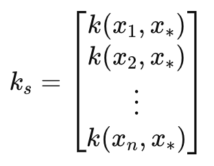
Where

• k(x i , y i ) is a Radial Basis Function between two values in the vectors x and y at index i. In our case, x and y are the same input time vector, thus both vectors are labelled x. x is usually the training data while y is a placeholder for the test data.
• k s is the covariance vector (or matrix in the even length-scale or number of projections exceeds 1) between the training data and the test point x∗.
• x 1 , x 2 ,…, xn, are the input training data points.
• x∗ is the input test data point where predictions are to be made.

This leads to the _k_ss matrix that in essence is a mirror image of the _k matrix, with the key difference being it is a covariance of the forecast time indices. Its dimensions therefore match the length-scale input parameter. It is instrumental in computing the uncertainty estimation portion of the forecast. It measures the variance over the forecast time indices before data is incorporated. This can be captured in a formula as:

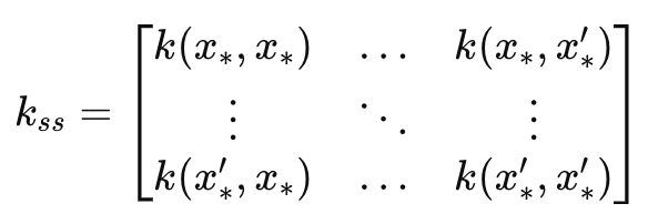
Where

• k ss is the covariance matrix of the test data points.
• x∗, x∗ ′are the input test data points where predictions are to be made.
• k(x∗,x∗′) is the kernel function applied to the pair of test points𝑥∗and𝑥∗′.

The _k_inv matrix as its name suggests is the inverse of the k matrix. Inversion of matrices is handled by inbuilt functions, however it is not fault free as often inversion may not be possible. That’s why, in our code, we check if the inverted matrix has any rows or columns. If none are present, it implies inversion has failed. This inversion is important for computing the weightings applied to the training data during forecasting. Alternative custom methods at performing this inversion like Cholesky could be considered (assuming it is not the inbuilt approach) however the coding of them as options is up to the reader.

The weight vector is used to combine outputs of training based on their covariance structure. _alpha determines how much influence new data points have on the prediction over the test/ length-scale points. We get alpha from the matrix product of the inverted k matrix and the raw old data for which we seek a forecast. This brings us to our objective, the _mu_star vector. This finally logs the forecasts over the input length-scale period based on the previous data that, whose size is defined by the input parameter m_past in the custom signal class. So, the number of projected means is determined by the length-scale which we refer to as m_next in the class and because vectors in MQL5 are not sorted as series (when copying and dealing with rates), the highest index of this forecast vector is projected to occur last while the zero index is meant to occur imminently. This implies that besides estimating what values are going to occur next in the series, we can project the trend that is to follow as well, depending on the size of the length-scale parameter. These projected values are also referred to as test points.

Once we have indicative means, the GP process also provides a sense of uncertainty around these values via the _sigma_star matrix. What it does capture is the covariance between different predictions at different points in the future or across the test-points. Because we are making a specific number of predictions, one for each test-point, we are only interested in the diagonal values of this matrix. We are not interested in the covariance between predictions. The formula for this matrix is given by:

Where

• k ss is the covariance matrix of the new data points as described above as _k_ss.
• k s is the covariance matrix between the new data points and the training data, also as already mentioned above as _k_s.
• K is the covariance matrix of the training data, the first matrix we defined.

From our equation above, the_vmatrix is indicated as the product between _k_s and the inverse K^-1. We are testing for 95% confidence, and thanks to the normal distribution tables this means for each test-point the upper bound value is the forecast mean plus 1.96 times the respective variance value in the matrix. Conversely, the lower bound value is the predicted mean minus 1.96 times the variance value from our _sigma_star matrix. This variance helps quantify our confidence with the mean predictions with, and this is important, larger values indicating greater uncertainty. So, the wider the confidence range (from upper bound value to lower bound value), the less confident one should be!

On a side note, but important point none-the-less, GP kernel computations involve finding matrix inversion and as already mentioned above this can be customized further by the reader by considering approaches like Cholesky’s decomposition in order to minimize errors and NaNs. Besides this, a common normalization technique that gets applied to the_k matrix early on in GP kernel process, is the addition of a small non-zero value across its diagonal so as to avert or prevent negative values showing up in the _sigma_star matrix. Recall this matrix has standard deviation values squared or the variance values, therefore all its values need to be positive. And bizarrely enough, an omission of this small addition across the _k matrix diagonal can lead to this matrix having negative values! So it’s an important step, and it is indicated in the listing of the get output function above.

So, our projections are giving us two things, the forecast and how ‘confident we should feel’ about this forecast. For this article, as can be seen below, we are performing tests by solely relying on the raw projection without factoring in the confidence levels as implied by the _sigma_star matrix. This in many ways is a huge under-representation of GP kernels, so, how could we factor in the implied confidence of a forecast in our custom signal? There are a variety of ways this can be accomplished, but even before these are considered, a quick solution would usually be outside of the custom signal class by using the magnitude of the confidence to guide position sizing.

This would imply we would, in addition to having a GP kernel in a custom signal class, we also have another GP kernel in a custom money management class. And in this situation, both the signal class and money management classes would have to be using similar input data sets and variance as well as length-scale parameters. However, within the custom signal class an easy incorporation would be to create a variances vector that copies the diagonal of the _sigma_star matrix, normalize it with our ‘SetOutput’ function and then determine the index with the lowest value. This index would then be used in the _mu_star vector to determine the custom signal’s condition. Since _mu_star is also normalized with the same function, then any values below 0.5 would map to negative changes which would be bearish while any values above 0.5 would be bullish.

Another method of using the quantified uncertainty of a forecast within a custom signal class could be if we take the weighted mean of all the forecasts or projections across all the test-points but use the normalized variance value as an inverse weight. It would be inverse, meaning we subtract it from one or invert it while adding a small value to the denominator. This inversion is important because, as emphasized above, a larger variance implies more uncertainty. This approaches at using uncertainty are only mentioned here but are not implemented in the code or during our test run. The reader is welcome to take this a step further by carrying out their own independent testing.

Data-Preprocessing and Normalization

GP kernels can be used for a variety of financial time series data broadly speaking this data can be in an absolute format such as absolute prices, or it can be in an incremental format such as changes in prices. For this article, we are going to test the GP kernel RBF with the latter. To this end, as can be seen in the ‘GetOutput’ listing above, we start by filling the ‘_past’ vector with the difference of two other vectors that both copied close prices from different points, 1 bar apart.

In addition to this, we could have normalized this price changes by converting them from their raw points and to have them in a -1.0 to +1.0 range. The ‘SetOutput’ function that is used for post-normalization or another custom method, could be used for this data-preprocessing as well. However, for our testing we are using the raw price changes in float (double) data format and only applying normalization to the forecast values (what we referred to as test-points above). This is performed with the ‘SetOutput’ function, whose code is listed below:

//+------------------------------------------------------------------+
//|
//+------------------------------------------------------------------+
void CSignalGauss::SetOutput(vector &Output)
{  vector _copy;
   _copy.Copy(Output);
   if(Output.HasNan() == 0 && _copy.Max() - _copy.Min() > 0.0)
   {  for (int i = 0; i < int(Output.Size()); i++)
      {  if(_copy[i] >= 0.0)
         {  Output[i] = 0.5 + (0.5 * ((_copy[i] - _copy.Min()) / (_copy.Max() - _copy.Min())));
         }
         else if(_copy[i] < 0.0)
         {  Output[i] = (0.5 * ((_copy[i] - _copy.Min()) / (_copy.Max() - _copy.Min())));
         }
      }
   }
   else
   {  Output.Fill(0.5);
   }
}

We have used this normalization in previous articles within this series and all that we are doing is re-scaling the projected vector values to be in the 0.0 to +1.0 range with the major caveat of anything less than 0.5 would have been negative in the de-normalized series while anything above 0.5 would have been positive.

Testing and Evaluation

For our test runs on a GP kernel RBF we are testing the pair EURUSD for the year 2023 on the daily time frame. As is often the case, but not always, these settings are got from a very short optimization stint, and they are not verified with a forward walk. Application of our wizard assembled Expert Advisor to real market conditions will require more independent diligence on the part of the reader to ensure that extensive testing on more history and with forward walks (cross-validation) is performed. The results of our run are below:

Conclusion

In conclusion, we have looked at Gaussian Process kernels as a potential signal to a trade system. ‘Gaussian’ often invokes random or the presumption that a system that is used assumes its environment is random, and therefore it is betting on 50–50 odds to make a buck. However, their proponents make the case that they use a provided data sample to forecast over a predefined period with a probabilistic framework. This method, it is argued, allows more flexibility since no assumptions are made to what the studied data adheres to (i.e. it is non-parametric). The only over-arching assumption is that the data follows a Gaussian distribution. Thus, why uncertainty is incorporated in the process and results, it argued the process is not random-centric.

In addition, from our coding and testing of the Gaussian Process kernels we have not exploited the quantification of uncertainty which one would argue sets it apart from other forecasting methods. With this said, the use and reliance on normal-distributions does raise the question of whether Gaussian Process kernels are meant to be used independently or work best when paired with an alternative signal. The MQL5 wizard, for which new readers can find guidance here and here, does easily allow more than one signal to be tested in a single Expert Advisor since each selected signal can be optimized to a suitable weighting. What alternative signal is worth pairing with these kernels? Well the best answer to this question can only be provided by the reader from his own testing, however if I were to suggest then it should be oscillators like RSI, or the stochastic oscillator or on-balance volume and even some news sentiment indicators. In addition, indicators like simple moving averages, moving average cross-overs, Price channel and indicators in general with a substantial lag may not work well when paired with Gaussian Process kernels.

We have also examined only one type of kernel, the Radial Basis Function, the other formats will be examined in coming articles in altered settings.