Reimagining Classic Strategies (Part V): Multiple Symbol Analysis on USDZAR

Introduction

There are innumerable ways we can integrate AI into our trading strategies, but unfortunately, we cannot evaluate each one before we decide which one to trust with our capital. Today, we revisit a popular trading strategy of multiple symbol analysis to determine if we can improve the strategy using AI. We will provide you with the information you need to arrive at an informed decision on whether this strategy is suitable for your investor profile.

Overview of the Trading Strategy

Trading strategies that employ multiple symbol analysis are mainly rooted in the correlation that is observed between the basket of symbols. Correlation is a measure of linear dependency between two variables. However, correlation is often mistaken for an indication of a relationship between two variables, which may not always be the case.   

Traders worldwide have taken advantage of their fundamental understanding of correlated assets to guide their investment decisions, measure risk levels and even as an exit signal. For example, let us consider the USDZAR currency pair. The American government is one of the leading exporters of oil in the world, while on the other hand, the South African government is the world’s largest exporter of gold.

Since these commodities contribute a significant proportion to the Gross Domestic Product of these two countries, one could naturally expect that the price levels of these commodities may explain some of the variance in the USDZAR currency pair. So if oil is performing better than gold in the spot market, we may expect the Dollar to be stronger than the Rand and vice versa.

Overview of the Methodology

For us to assess the relationship, we exported all our market data from our MetaTrader 5 terminal using a script written in MQL5. We trained various models using 2 groups of possible inputs for the models:

1. Ordinary OHLC quotes on the USDZAR.
2. A combination of oil and gold prices.

From the data collected, it appears that oil has stronger correlation levels with the UDZAR currency pair than gold.

Since our data were on different scales, we standardized and normalized the data before training. We performed 10-fold cross validation without random shuffling to compare our accuracy across the different sets of inputs.

Our findings suggest that the first group may yield the lowest error. The best performing model was the linear regression using Ordinary OHLC data. However, in the latter group, 2, the best performing model was the KNeigborsRegressor algorithm.

We successfully performed hyperparameter tuning using 500 iterations of a randomized search over 5 parameters of the model. We tested for overfitting by comparing the error levels of our customized model against a default model on a validation set that was held out during optimization, after training both models on equivalent training sets, we outperformed the default model on the validation set.

Finally, we exported our customized model to ONNX format, and integrated it into our Expert Advisor in MQL5.

Data Extraction

I’ve built a handy script to help extract the required data from your MetaTrader 5 terminal, simply drag and drop the script onto your desired symbol, and it will extract the data for you and place it in the path: “\MetaTrader 5\MQL5\Files\..”

//+------------------------------------------------------------------+
//|                                                      ProjectName |
//|                                      Copyright 2020, CompanyName |
//|                                       http://www.companyname.net |
//+------------------------------------------------------------------+
#property copyright "Gamuchirai Zororo Ndawana"
#property link      "https://www.mql5.com/en/users/gamuchiraindawa"
#property version   "1.00"
#property script_show_inputs

//---Amount of data requested
input int size = 100000; //How much data should we fetch?

//+------------------------------------------------------------------+
//|                                                                  |
//+------------------------------------------------------------------+
void OnStart()
  {
//---File name
   string file_name = "Market Data " + Symbol() + ".csv";

//---Write to file
   int file_handle=FileOpen(file_name,FILE_WRITE|FILE_ANSI|FILE_CSV,",");

   for(int i= size;i>=0;i--)
     {
      if(i == size)
        {
         FileWrite(file_handle,"Time","Open","High","Low","Close");
        }

      else
        {
         FileWrite(file_handle,iTime(Symbol(),PERIOD_CURRENT,i),
                   iOpen(Symbol(),PERIOD_CURRENT,i),
                   iHigh(Symbol(),PERIOD_CURRENT,i),
                   iLow(Symbol(),PERIOD_CURRENT,i),
                   iClose(Symbol(),PERIOD_CURRENT,i));
        }
     }

  }
//+------------------------------------------------------------------+

Exploratory Data Analysis in Python

We begin by importing standard libraries.

#Libraries
import pandas as pd
import numpy as np
import seaborn as sns

Now let us read in the data we extracted earlier.

#Dollar VS Rand
USDZAR = pd.read_csv("/home/volatily/market_data/Market Data USDZAR.csv")
#US Oil
USOIL = pd.read_csv("/home/volatily/market_data/Market Data US Oil.csv")
#SA Gold
SAGOLD = pd.read_csv("/home/volatily/market_data/Market Data XAUUSD.csv")

Inspecting the data.

USOIL

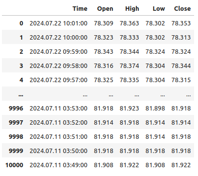
Fig 1: Our data is running backwards in time

Notice that our timestamps are running from near the present and further back into the past, this is undesirable for machine learning tasks. Let us reverse the order of the data so that we are forecasting into the future, and not into the past.

#Format the data
USDZAR = USDZAR[::-1]
USOIL = USOIL[::-1]
SAGOLD = SAGOLD[::-1]

Before we can merge our datasets, let us first ensure that they all use the date column as indexes. By doing so, we can be sure that we only select days shared by all datasets, in the correct chronological order.

#Set the indexes
USOIL = USOIL.set_index("Time")
SAGOLD = SAGOLD.set_index("Time")
USDZAR = USDZAR.set_index("Time")

Merging the datasets.

#Merge the dataframes
merged_df = pd.merge(USOIL,SAGOLD,how="inner",left_index=True,right_index=True,suffixes=(" US OIL"," SA GOLD"))
merged_df = pd.merge(merged_df,USDZAR,how="inner",left_index=True,right_index=True)

Defining the forecast horizon.

#Define the forecast horizon
look_ahead = 10

The target will be the future close price of the USDZAR pair, we will also include a binary target for visualization purposes.

#Label the data
merged_df["Target"] = merged_df["Close"].shift(-look_ahead)
merged_df["Binary Target"] = 0
merged_df.loc[merged_df["Close"] < merged_df["Target"],"Binary Target"] = 1

Let us drop any empty rows.

#Drop empty rows
merged_df.dropna(inplace=True)

Observe the correlation levels.

#Let's observe the correlation levels
merged_df.corr()

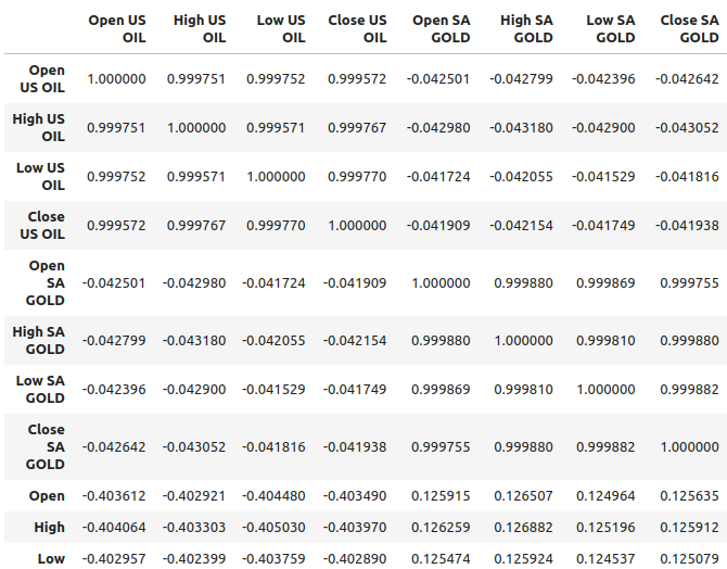
Fig 2: Correlation levels in our dataset

Oil appears to be demonstrating relatively stronger correlation levels with the USDZAR pair, approximately -0.4, while gold has relatively weaker correlation levels with the currency pair, approximately 0.1. It is important to remember that correlation does not always imply there is a relationship between the variables, sometimes correlation results from a common cause that is affecting both variables.

For example, historically, the relationship between gold and the Dollar was inverted. Whenever the Dollar was depreciating, traders would take their money out of the dollar and invest it in gold instead. This historically caused gold prices to rally whenever the dollar was performing poorly. So the common cause, in this simple example, would be the traders who were participating in both markets.

Scatter plots help us visualize the relationship between 2 variables, so we created a scatter plot of oil prices against gold prices and colored the points depending on whether price levels of the USDZAR appreciated (red) or depreciated (green). As one can see, there is no clear level of separation in the data. In fact, none of the scatter plots we created suggest a strong relationship.

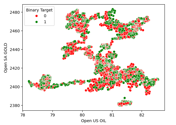
Fig 3: A scatterplot of gold prices against oil prices

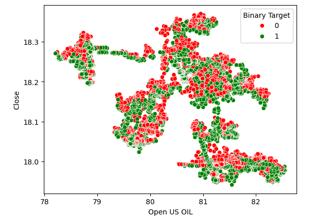
Fig 4:Scatterplot of oil prices against the USDZAR close price

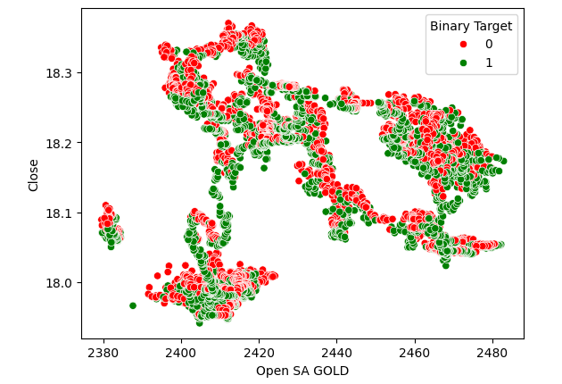
Fig 5:A scatter plot of gold prices against the USDZAR close

Modelling The Relationship

Let us reset the index of our data set so that we can perform cross validation.

#Reset the index
merged_df.reset_index(inplace=True)

Now we shall import the libraries we need to model the relationship in the data.

#Import the libraries we need
from sklearn.linear_model import LinearRegression
from sklearn.linear_model import Lasso
from sklearn.ensemble import GradientBoostingRegressor
from sklearn.ensemble import RandomForestRegressor
from sklearn.ensemble import AdaBoostRegressor
from sklearn.ensemble import BaggingRegressor
from sklearn.neighbors import KNeighborsRegressor
from sklearn.svm import LinearSVR
from sklearn.neural_network import MLPRegressor
from sklearn.model_selection import TimeSeriesSplit
from sklearn.metrics import root_mean_squared_error
from sklearn.preprocessing import RobustScaler

Defining the predictors and the target.

#Define the predictors
normal_predictors = ["Open","High","Low","Close"]
oil_gold_predictors = ["Open US OIL","High US OIL","Low US OIL","Close US OIL","Open SA GOLD","High SA GOLD","Low SA GOLD","Close SA GOLD"]
target = "Target"

Scaling the data.

#Scale the data
all_predictors = normal_predictors + oil_gold_predictors
scaler = RobustScaler()
scaled_data = pd.DataFrame(scaler.fit_transform(merged_df.loc[:,all_predictors]),columns=all_predictors,index=np.arange(0,merged_df.shape[0]))

Initializing the models.

#Now prepare the models
models = [
        LinearRegression(),
        Lasso(),
        GradientBoostingRegressor(),
        RandomForestRegressor(),
        AdaBoostRegressor(),
        BaggingRegressor(),
        KNeighborsRegressor(),
        LinearSVR(),
        MLPRegressor(hidden_layer_sizes=(10,5),early_stopping=True),
        MLPRegressor(hidden_layer_sizes=(50,15),early_stopping=True)
]

columns = [
        "Linear Regression",
        "Lasso",
        "Gradient Boosting Regressor",
        "Random Forest Regressor",
        "AdaBoost Regressor",
        "Bagging Regressor",
        "KNeighbors Regressor",
        "Linear SVR",
        "Small Neural Network",
        "Large Neural Network"
]

Instantiating the time-series cross-validation object.

#Prepare the time-series split object
splits = 10
tscv = TimeSeriesSplit(n_splits=splits,gap=look_ahead)

Creating a data frame to store our error levels.

#Prepare the dataframes to store the error levels
normal_error = pd.DataFrame(columns=columns,index=np.arange(0,splits))
new_error = pd.DataFrame(columns=columns,index=np.arange(0,splits))

Now we will perform cross-validation using a nested for loop. The first loop iterates over our list of models, while the second loop cross validates each model and stores the error levels.

#First we iterate over all the models we have available
for j in np.arange(0,len(models)):
        #Now we have to perform cross validation with each model
        for i,(train,test) in enumerate(tscv.split(scaled_data)):
        #Get the data
        X_train = scaled_data.loc[train[0]:train[-1],oil_gold_predictors]
        X_test = scaled_data.loc[test[0]:test[-1],oil_gold_predictors]
        y_train = merged_df.loc[train[0]:train[-1],target]
        y_test = merged_df.loc[test[0]:test[-1],target]
        #Fit the model
        models[j].fit(X_train,y_train)
        #Measure the error
        new_error.iloc[i,j] = root_mean_squared_error(y_test,models[j].predict(X_test))

Our error levels using the ordinary model inputs.

normal_error

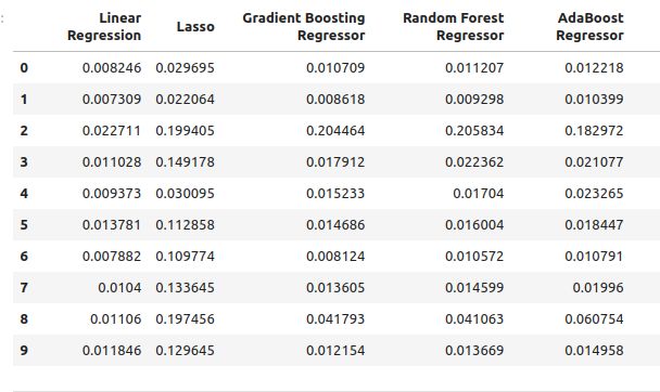
Fig 6: Our error levels when forecasting using OHLC predictors

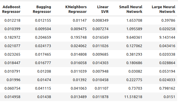
Fig 7: Our error levels when forecasting using OHLC predictors II

Now take a look at our error levels using just oil and gold prices.

new_error

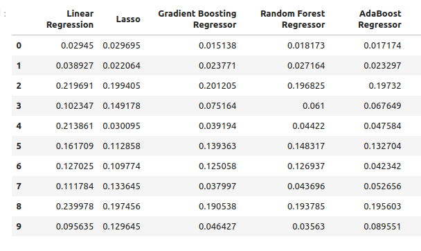
Fig 8: Our accuracy levels when forecasting using oil and gold prices

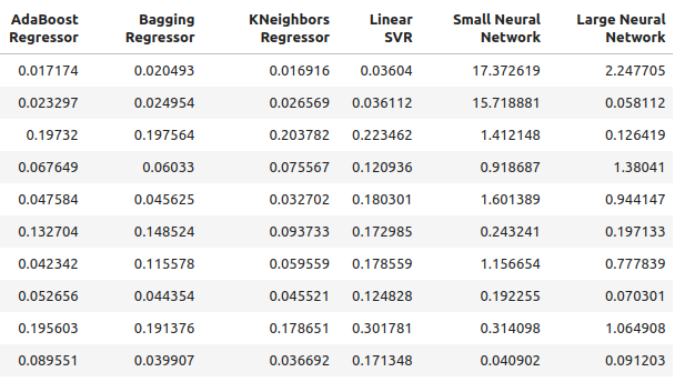
Fig 9: Our accuracy levels when forecasting using oil and gold prices II

Let’s see our average performance from each model using ordinary predictors.

#Let's see our average performance on the normal dataset
for i in (np.arange(0,normal_error.shape[0])):
        print(f"{models[i]} normal error {((normal_error.iloc[:,i].mean()))}")

LinearRegression() normal error 0.01136361865358375
Lasso() normal error 0.11138143304314707
GradientBoostingRegressor() normal error 0.03472997520534606
RandomForestRegressor() normal error 0.03616484012058101
AdaBoostRegressor() normal error 0.037484107657877755
BaggingRegressor() normal error 0.03670486223028821
KNeighborsRegressor() normal error 0.035113189373409175
LinearSVR() normal error 0.01085610361276552
MLPRegressor(early_stopping=True, hidden_layer_sizes=(10, 5)) normal error 2.558754334716706
MLPRegressor(early_stopping=True, hidden_layer_sizes=(50, 15)) normal error 1.0544369296125597

Now we will assess our average performance using the new predictors.

#Let's see our average performance on the new dataset
for i in (np.arange(0,normal_error.shape[0])):
        print(f"{models[i]} normal error {((new_error.iloc[:,i].mean()))}")

LinearRegression() normal error 0.13404065973045615
Lasso() normal error 0.11138143304314707
GradientBoostingRegressor() normal error 0.0893855335909897
RandomForestRegressor() normal error 0.08957454602573789
AdaBoostRegressor() normal error 0.08658796789785872
BaggingRegressor() normal error 0.08887059320664067
KNeighborsRegressor() normal error 0.07696901077705855
LinearSVR() normal error 0.15463529064256165
MLPRegressor(early_stopping=True, hidden_layer_sizes=(10, 5)) normal error 3.8970873719426784
MLPRegressor(early_stopping=True, hidden_layer_sizes=(50, 15)) normal error 0.6958177634524169

Let's observe the changes in accuracy.

#Let's see our average performance on the normal dataset
for i in (np.arange(0,normal_error.shape[0])):
    print(f"{models[i]} changed by {((normal_error.iloc[:,i].mean()-new_error.iloc[:,i].mean()))/normal_error.iloc[:,i].mean()}%")

LinearRegression() changed by -10.795596439535894%
Lasso() changed by 0.0%
GradientBoostingRegressor() changed by -1.573728690057642%
RandomForestRegressor() changed by -1.4768406476311784%
AdaBoostRegressor() changed by -1.3099914419240863%
BaggingRegressor() changed by -1.421221271695885%
KNeighborsRegressor() changed by -1.1920256220116057%
LinearSVR() changed by -13.244087580439862%
MLPRegressor(early_stopping=True, hidden_layer_sizes=(10, 5)) changed by -0.5230408480672479%
MLPRegressor(early_stopping=True, hidden_layer_sizes=(50, 15)) changed by 0.34010489967561475%

Feature Selection

Our best performing model from the oil and gold predictors is the KNeighbors regressor, let us see which features are most important to it.

#Our best performing model was the KNeighbors Regressor
#Let us perform feature selection to test how stable the relationship is
from mlxtend.feature_selection import SequentialFeatureSelector as SFS

Create a new instance of the model.

#Let us select our best model
model = KNeighborsRegressor()

We will use forward selection to identify the most important features for our model. We will now give our model access to all the predictors at once.

#Create the sequential selector object
sfs1 = SFS(
        model,
        k_features=(1,len(all_predictors)),
        forward=True,
        scoring="neg_mean_squared_error",
        cv=10,
        n_jobs=-1
)

Fitting the sequential feature selector.

#Fit the sequential selector
sfs1 = sfs1.fit(scaled_data.loc[:,all_predictors],merged_df.loc[:,"Target"])

Observing the best features selected by the algorithm may lead us to conclude that neither oil nor gold prices are of much use when forecasting the USDZAR because our algorithm only selected 3 features that were quotes of open, low and close price of the USDZAR.

#Now let us see which predictors were selected
sfs1.k_feature_names_

('Open', 'Low', 'Close')

Hyperparameter Tuning

Let us attempt to perform hyperparameter tuning using the RandomizedSearchCV module of scikit-learn. The algorithm helps us sample a response surface that may be too large to sample entirely. When we use models with numerous parameters, the total combinations of inputs grows at a significantly fast rate. Therefore, we prefer the randomized search algorithm when we are dealing with many parameters that have many possible values.

The algorithm provides a trade-off between accuracy of results and time of computation. This trade-off is controlled by adjusting the number of iterations we allow. Note that due to the random nature of the algorithm, it may be challenging to exactly reproduce the results demonstrated in this article.

Import the scikit-learn module.
#Now we will load the libraries we need
from sklearn.model_selection import RandomizedSearchCV

Prepare dedicated train, and test sets.

#Let us see if we can tune the model
#First we will create train test splits
train_X = scaled_data.loc[:(scaled_data.shape[0]//2),:]
train_y = merged_df.loc[:(merged_df.shape[0]//2),"Target"]

test_X = scaled_data.loc[(scaled_data.shape[0]//2):,:]
test_y = merged_df.loc[(merged_df.shape[0]//2):,"Target"]

To perform parameter tuning, we need to pass an estimator that implements the scikit-learn interface, followed by a dictionary that contains keys that correspond to the parameters of the estimator and values that correspond to the range of allowed inputs for each parameter, from there we specify that we would like to perform 5-fold cross-validation, and then we have to specify the scoring metric as negative mean squared error.

#Create the tuning object
rs = RandomizedSearchCV(KNeighborsRegressor(n_jobs=-1),{
        "n_neighbors": [1,2,3,4,5,8,10,16,20,30,60,100],
        "weights":["uniform","distance"],
        "leaf_size":[1,2,3,4,5,10,15,20,40,60,90],
        "algorithm":["ball_tree","kd_tree"],
        "p":[1,2,3,4,5,6,7,8]
},cv=5,n_iter=500,return_train_score=False,scoring="neg_mean_squared_error")

Performing parameter tuning on the training set.

#Let's perform the hyperparameter tuning
rs.fit(train_X,train_y)

Looking at the results we obtained, from best to worst.

#Let's store the results from our hyperparameter tuning
tuning_results = pd.DataFrame(rs.cv_results_)
tuning_results.loc[:,["param_n_neighbors","param_weights","param_leaf_size","param_algorithm","param_p","mean_test_score"]].sort_values(by="mean_test_score",ascending=False)

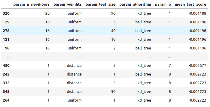
Fig 10: The results of tuning our best model

These are the best parameters we found.

#The best parameters we came across
rs.best_params_

{'weights': 'distance',
 'p': 1,
 'n_neighbors': 4,
 'leaf_size': 15,
 'algorithm': 'ball_tree'}

Checking for Overfitting

Let’s get ready to compare our customized and default models. Both models will be trained on identical training sets. If the default model outperforms our customized model on the validation set, then it may be a sign we over fit the training data. However, if our customized model performs better, then it may suggest we have successfully tuned the model parameters without over fitting.

#Create instances of the default model and the custmoized model
default_model = KNeighborsRegressor()
customized_model = KNeighborsRegressor(p=rs.best_params_["p"],weights=rs.best_params_["weights"],n_neighbors=rs.best_params_["n_neighbors"],leaf_size=rs.best_params_["leaf_size"],algorithm=rs.best_params_["algorithm"])

Let’s measure the accuracy of the default model.

#Measure the accuracy of the default model
default_model.fit(train_X,train_y)
root_mean_squared_error(test_y,default_model.predict(test_X))

0.06633226373900612

Now the accuracy of the customized model.

#Measure the accuracy of the customized model
customized_model.fit(train_X,train_y)
root_mean_squared_error(test_y,customized_model.predict(test_X))

0.04334616246844129

It appears that we have tuned the model well without overfitting! Let us now get ready to export our customized model to ONNX format.

Exporting to ONNX Format

Open Neural Network Exchange (ONNX) is an interoperable framework for building and deploying machine learning models in a language-agnostic manner. By using ONNX, our machine learning models can be easily used in any programming language so long as that language supports the ONNX API. At the time of writing, the ONNX API is being developed and maintained by a consortium of the largest companies in the world.

Import the libraries we need
#Let's prepare to export the customized model to ONNX format
import onnx
from skl2onnx import convert_sklearn
from skl2onnx.common.data_types import FloatTensorType

We need to ensure that our data is scaled and normalized in a way that we can reproduce in the MetaTrader 5 terminal. Therefore, we will perform a standard transform that we can always perform in our terminal later on. We will subtract the mean value of each column, this will center our data. And then we will divide each value by the standard deviation of its particular column, this will help our model better appreciate changes across variables on different scales.

#Train the model on all the data we have
#But before doing that we need to first scale the data in a way we can repeat in MQL5
scale_factors = pd.DataFrame(columns=all_predictors,index=["mean","standard deviation"])
for i in np.arange(0,len(all_predictors)):
        scale_factors.iloc[0,i] = merged_df.loc[:,all_predictors[i]].mean()
        scale_factors.iloc[1,i] = merged_df.loc[:,all_predictors[i]].std()
scale_factors

Fig 12: Some of the values we will use to scale and standardize our data, not all columns are being displayed

Now let us perform the normalization and standardization.

for i in all_predictors:
        merged_df.loc[:,i] = (merged_df.loc[:,i] - merged_df.loc[:,i].mean()) / merged_df.loc[:,i].std()

Let us look at our data now.

merged_df

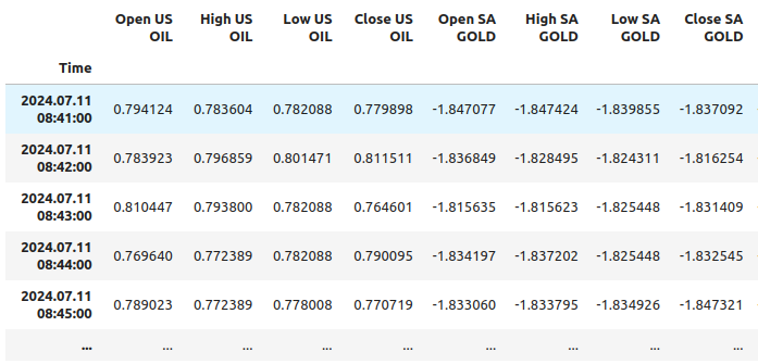
Fig 11: What our data looks like after scaling, not all columns are being shown

Initialize our customized model.

customized_model = KNeighborsRegressor(p=rs.best_params_["p"],weights=rs.best_params_["weights"],n_neighbors=rs.best_params_["n_neighbors"],leaf_size=rs.best_params_["leaf_size"],algorithm=rs.best_params_["algorithm"])
customized_model.fit(merged_df.loc[:,all_predictors],merged_df.loc[:,"Target"])

Define the input shape of our model.

#Define the input shape and type
initial_type = [("float_tensor_type",FloatTensorType([1,train_X.shape[1]]))]

Create the ONNX representation.

#Create an ONNX representation
onnx_model = convert_sklearn(customized_model,initial_types=initial_type)

Save the ONNX model.

#Store the ONNX model
onnx_model_name = "USDZAR_FLOAT_M1.onnx"
onnx.save_model(onnx_model,onnx_model_name)

Visualizing the ONNX Model

Netron is an open-source visualizer for machine learning models. Netron extends support to many different frameworks besides ONNX like as Keras. We will use netron to ensure that our ONNX model has the input and output shape we were expecting.

Import the netron module.

#Let's visualize the model in netron
import netron

Now we can visualize the model using netron.

#Run netron
netron.start(onnx_model_name)

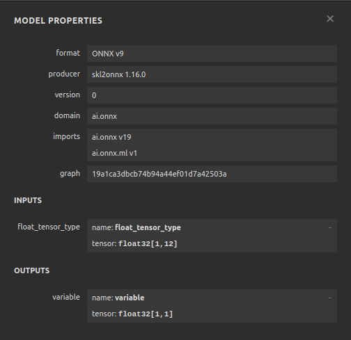
Fig 12: The specifications of our ONNX model

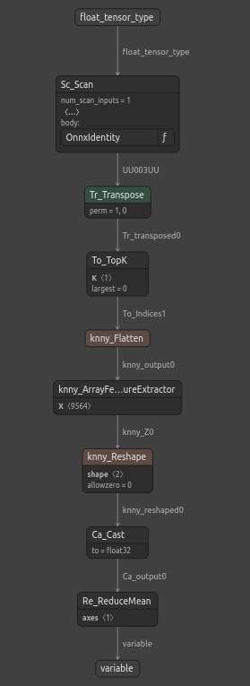
Fig 13: The structure of our ONNX model

Our ONNX model is meeting our expectations, the input and output shape are accurately where we expect them to be. We can now move on to building an Expert Advisor on top of our ONNX model.

Implementation in MQL5

We can now begin building our Expert Advisor, let us start by first integrating our ONNX model into our application. By specifying the ONNX file as a resource, the ONNX file will be included in the compiled program with the .ex5 extension.

//+------------------------------------------------------------------+
//|                                                       USDZAR.mq5 |
//|                                        Gamuchirai Zororo Ndawana |
//|                          https://www.mql5.com/en/gamuchiraindawa |
//+------------------------------------------------------------------+
#property copyright "Gamuchirai Zororo Ndawana"
#property link      "https://www.mql5.com/en/gamuchiraindawa"
#property version   "1.00"

//+-----------------------------------------------------------------+
//| Require the ONNX file                                           |
//+-----------------------------------------------------------------+
#resource "\\Files\\USDZAR_FLOAT_M1.onnx" as const uchar onnx_model_buffer[];

Now we will import the trade library.

//+-----------------------------------------------------------------+
//| Libraries we need                                               |
//+-----------------------------------------------------------------+
#include <Trade/Trade.mqh>
CTrade Trade;

Let us define inputs the end user can control.

//+------------------------------------------------------------------+
//| Inputs                                                           |
//+------------------------------------------------------------------+
double input sl_width = 0.4;              //How tight should our stop loss be?
int input lot_multiple = 10;              //How many times bigger than minimum lot should we enter?
double input max_risk = 10;               //After how much profit/loss should we close?

Now we need a few global variables.

//+------------------------------------------------------------------+
//| Global Variables                                                 |
//+------------------------------------------------------------------+
long onnx_model;                          //Our onnx model
double mean_values[12],std_values[12];    //The scaling factors we used for our data
vector model_inputs = vector::Zeros(12);  //Our model's inputs
vector model_forecast = vector::Zeros(1); //Our model's output
double bid,ask;                           //Market prices
double minimum_volume;                    //Smallest lot size
double state = 0;                         //0 means we have no positions, 1 means we have buy position, 2 means we have sell position.

Let us now define helper functions for tasks that we may need to perform repeatedly. First, let us control our risk levels, if the total profit/loss exceeded our defined risk levels, we will automatically close the position.

//+------------------------------------------------------------------+
//| Check if we have reached our risk level                          |
//+------------------------------------------------------------------+
void check_risk_level(void)
  {
//--- Check if we have surpassed our maximum risk level
   if(MathAbs(PositionGetDouble(POSITION_PROFIT)) > max_risk)
     {
      //--- We should close our positions
      Trade.PositionClose("USDZAR");
     }
  }

Since we have an integrated AI system, let us use it to detect reversals. If our system predicts that price will move against us, we will close the position and alert the end user that a potential reversal has been detected.

//+------------------------------------------------------------------+
//| Check if there is a reversal may be coming                       |
//+------------------------------------------------------------------+
void check_reversal(void)
  {
   if(((state == 1) && (model_forecast[0] < iClose("USDZAR",PERIOD_M1,0))) ||((state == 2) && (model_forecast[0] > iClose("USDZAR",PERIOD_M1,0))))
     {
      //--- There may be a reversal coming
      Trade.PositionClose("USDZAR");
      //--- Give the user feedback
      Alert("Potential reversal detected");
     }
  }

We now need a function to find entry opportunities for us. We will only consider an entry to be valid if our model’s prediction aligns with the changes in price levels on higher time frames. 

//+------------------------------------------------------------------+
//| Find an entry opportunity                                        |
//+------------------------------------------------------------------+
void find_entry(void)
  {
//---Check for the change in price on higher timeframes
   if(iClose("USDZAR",PERIOD_D1,0) > iClose("USDZAR",PERIOD_D1,21))
     {
      //--- We're looking for buy oppurtunities
      if(model_forecast[0] > iClose("USDZAR",PERIOD_M1,0))
        {
         //--- Open the position
         Trade.Buy(minimum_volume,"USDZAR",ask,(ask - sl_width),(ask + sl_width),"USDZAR AI");
         //--- Update the system state
         state = 1;
        }
     }
//---Check for the change in price on higher timeframes
   else
      if(iClose("USDZAR",PERIOD_D1,0) < iClose("USDZAR",PERIOD_D1,21))
        {
         //--- We're looking for sell oppurtunities
         if(model_forecast[0] < iClose("USDZAR",PERIOD_M1,0))
           {
            //--- Open sell position
            Trade.Sell(minimum_volume,"USDZAR",bid,(bid + sl_width),(bid - sl_width),"USDZAR AI");
            //--- Update the system state
            state = 2;
           }
        }
  }

Now we need a function to fetch a prediction from our model. To do so, we first need to fetch current market prices and then transform them by subtracting the mean and dividing by the standard deviation.

//+------------------------------------------------------------------+
//| Obtain a forecast from our model                                 |
//+------------------------------------------------------------------+
void model_predict(void)
  {
//Let's fetch our model's inputs
//--- USDZAR
   model_inputs[0] = ((iOpen("USDZAR",PERIOD_M1,0) - mean_values[0]) / std_values[0]);
   model_inputs[1] = ((iHigh("USDZAR",PERIOD_M1,0) - mean_values[1]) / std_values[1]);
   model_inputs[2] = ((iLow("USDZAR",PERIOD_M1,0) - mean_values[2]) / std_values[2]);
   model_inputs[3] = ((iClose("USDZAR",PERIOD_M1,0) - mean_values[3]) / std_values[3]);
//--- XTI OIL US
   model_inputs[4] = ((iOpen("XTIUSD",PERIOD_M1,0) - mean_values[4]) / std_values[4]);
   model_inputs[5] = ((iHigh("XTIUSD",PERIOD_M1,0) - mean_values[5]) / std_values[5]);
   model_inputs[6] = ((iLow("XTIUSD",PERIOD_M1,0) - mean_values[6]) / std_values[6]);
   model_inputs[7] = ((iClose("XTIUSD",PERIOD_M1,0) - mean_values[7]) / std_values[7]);
//--- GOLD SA
   model_inputs[8] = ((iOpen("XAUUSD",PERIOD_M1,0) - mean_values[8]) / std_values[8]);
   model_inputs[9] = ((iHigh("XAUUSD",PERIOD_M1,0) - mean_values[9]) / std_values[9]);
   model_inputs[10] = ((iLow("XAUUSD",PERIOD_M1,0) - mean_values[10]) / std_values[10]);
   model_inputs[11] = ((iClose("XAUUSD",PERIOD_M1,0) - mean_values[11]) / std_values[11]);
//--- Get a prediction
   OnnxRun(onnx_model,ONNX_DEFAULT,model_inputs,model_forecast);
  }

Since we are analyzing multiple symbols, we need to add them to the market watch.

//+------------------------------------------------------------------+
//| Load the symbols we need and add them to the market watch        |
//+------------------------------------------------------------------+
void load_symbols(void)
  {
   SymbolSelect("XAUUSD",true);
   SymbolSelect("XTIUSD",true);
   SymbolSelect("USDZAR",true);
  }

We need a function responsible for loading our scaling factors, the mean and standard deviation of each column.

//+------------------------------------------------------------------+
//| Load the scale values                                            |
//+------------------------------------------------------------------+
void load_scale_values(void)
  {
//--- Mean
//--- USDZAR
   mean_values[0] = 18.14360511919699;
   mean_values[1] = 18.145737421580925;
   mean_values[2] = 18.141568574864074;
   mean_values[3] = 18.14362306984525;
//--- XTI US OIL
   mean_values[4] = 80.76956702216644;
   mean_values[5] = 80.7864452112087;
   mean_values[6] = 80.75236177331661;
   mean_values[7] = 80.76923546633206;
//--- GOLD SA
   mean_values[8] = 2430.5180384776245;
   mean_values[9] = 2430.878959640318;
   mean_values[10] = 2430.1509598494354;
   mean_values[11] = 2430.5204140526976;
//--- Standard Deviation
//--- USDZAR
   std_values[0] = 0.11301636249300206;
   std_values[1] = 0.11318116432297631;
   std_values[2] = 0.11288670156099372;
   std_values[3] = 0.11301994613848391;
//--- XTI US OIL
   std_values[4] = 0.9802409859148413;
   std_values[5] = 0.9807944310705999;
   std_values[6] = 0.9802449355481064;
   std_values[7] = 0.9805961626626833;
//--- GOLD SA
   std_values[8] = 26.397404261230328;
   std_values[9] = 26.414599597905003;
   std_values[10] = 26.377605644853944;
   std_values[11] = 26.395208330942864;
  }

Finally, we need a function responsible for loading our ONNX file.

//+------------------------------------------------------------------+
//| Load the onnx file from buffer                                   |
//+------------------------------------------------------------------+
bool load_onnx_file(void)
  {
//--- Create the model from the buffer
   onnx_model = OnnxCreateFromBuffer(onnx_model_buffer,ONNX_DEFAULT);

//--- The input size for our onnx model
   ulong input_shape [] = {1,12};

//--- Check if we have the right input size
   if(!OnnxSetInputShape(onnx_model,0,input_shape))
     {
      Comment("Incorrect input shape, the model has input shape ",OnnxGetInputCount(onnx_model));
      return(false);
     }

//--- The output size for our onnx model
   ulong output_shape [] = {1,1};

//--- Check if we have the right output size
   if(!OnnxSetOutputShape(onnx_model,0,output_shape))
     {
      Comment("Incorrect output shape, the model has output shape ",OnnxGetOutputCount(onnx_model));
      return(false);
     }

//--- Everything went fine
   return(true);
  }
//+------------------------------------------------------------------+

Now that we have defined these helper functions, we can begin using them in our Expert Advisor. First, let us define the behavior of our application whenever it is loaded for the first time. We will start by loading our ONNX model, getting the scaling values ready, and then we will fetch market data.

//+------------------------------------------------------------------+
//| Expert initialization function                                   |
//+------------------------------------------------------------------+
int OnInit()
  {
//--- Load the onnx file
   if(!load_onnx_file())
     {
      return(INIT_FAILED);
     }

//--- Load our scaling values
   load_scale_values();

//--- Add the symbols we need to the market watch
   load_symbols();

//--- The smallest lotsize we can use
   minimum_volume = SymbolInfoDouble("USDZAR",SYMBOL_VOLUME_MIN) * lot_multiple;

//--- Everything went fine
   return(INIT_SUCCEEDED);
  }

Whenever our program has been deactivated, we need to free up the resources that we are no longer using.

//+------------------------------------------------------------------+
//| Expert deinitialization function                                 |
//+------------------------------------------------------------------+
void OnDeinit(const int reason)
  {
//--- Release the resources we used for our onnx model
   OnnxRelease(onnx_model);

//--- Remove the expert advisor
   ExpertRemove();
  }

Finally, whenever price changes, we need to fetch a new forecast from our model, get updated market prices and then either open a new position or manage the positions we have currently open.

//+------------------------------------------------------------------+
//| Expert tick function                                             |
//+------------------------------------------------------------------+
void OnTick()
  {
//--- We always need a forecast from our model
   model_predict();
//--- Fetch market prices
   bid = SymbolInfoDouble("USDZAR",SYMBOL_BID);
   ask = SymbolInfoDouble("USDZAR",SYMBOL_ASK);

//--- If we have no open positions, find an entry
   if(PositionsTotal() == 0)
     {
      //--- Find an entry
      find_entry();
      //--- Reset the system state
      state = 0;
     }

//--- If we have open postitions, manage them
   else
     {
      //--- Check for a reveral warning from our AI
      check_reversal();
      //--- Check if we have not reached our max risk levels
      check_risk_level();
     }

  }

Putting all of this together, we can now observe our program in action. 

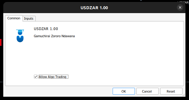
Fig 17: Our Expert Advisor

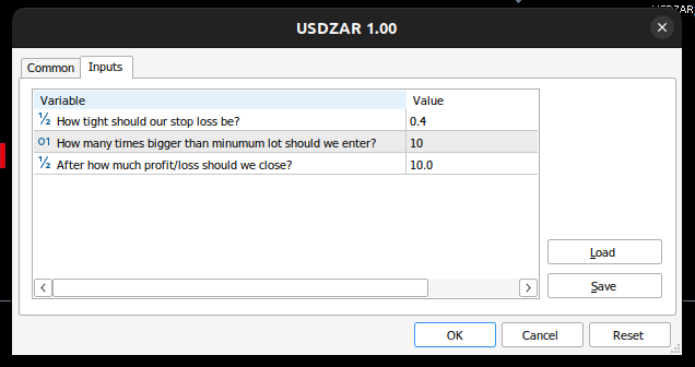
Fig 14: The inputs for our expert advisor

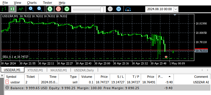
Fig 15: Our program in action

Conclusion

In this article, we have demonstrated how you can build a multiple symbol Expert Advisor powered with AI. Although we obtained lower error levels using ordinary OHLC, this does not necessarily mean that the same will be true for all the symbols you have in your MetaTrader 5 terminal, there may exist a basket of different symbols that may produce lower error than the USDZAR OHLC quotes.