MQL5 Wizard Techniques you should know (Part 31): Selecting the Loss Function

Introduction

MQL5 wizard can be a test bed for a wide variety of ideas, as we have covered so far in these series. And every once in a while, one is presented with a custom signal that has more than one way of being implemented. We looked at this scenario in the 2 articles about learning rates, as well as the last article on batch normalization. Each of those aspects to machine learning presented more than one potential custom signal, as was discussed. The loss , also by virtue of having multiple formats, is in a similar situation.

The way in which a test run result is compared to its target does not have a single method. If we consider the enumerations available in ENUM_LOSS_FUNCTION enumeration in MQL5, they are 14, and this list is not even exhaustive. Does this mean that every one of them offers a distinct way at training in machine learning? Probably not, but the point is there are differences, some nuanced, and these differences can often imply you need to carefully select your loss function depending on the nature of the network or algorithm you are training.

Besides the loss function though, one could consider using the ENUM_REGRESSION_METRIC but this, which is more statistical related, would be inappropriate as it better serves as a post-training metric for assessing performance of a machine learning algorithm. So particularly in instances where the final output has more than one dimension then this metric enumeration would be very helpful. This article though is focusing on the objective function.

And the selection of the appropriate loss measure is vital because in principle, neural-networks (our machine learning algorithm for this article) could fall in the category of regressors versus classifiers, or they are in the type of supervised versus unsupervised. In addition, paradigms such as reinforcement learning could require a multi-faceted approach at using and applying the loss function.

So, loss functions can be applied in various ways not just because there are many formats, but also there is a variety of ‘problems’ (neural network types) to solve. In resolving these problems or in training, the loss function primarily quantifies how far off the tested parameters are from their intended target, a process also referred to as supervised learning.

However, even though with the loss function it always seems intuitive that they are meant for supervised training; the question of the ideal loss function for unsupervised learning could seem off. None-the-less, even in unsupervised settings such as Kohonen maps or clustering, there is always a need to have a standardized metric when measuring gaps or distance across multi-dimensioned data and the loss function would fill this void.

Overview of Loss Functions

So MQL5 offers up to 14 different methods of quantifying the loss function, and we will touch on all before considering application cases. For our purpose, loss is used to imply loss-gradient and the expected outputs of this are vectors, not scalar values. Also, MQL5 code that implements these formulae will not be shared because they are ALL run from in-built vector functions. A simple script for testing out the various loss functions is given below:

#property  script_show_inputs
input ENUM_LOSS_FUNCTION __loss = LOSS_HUBER;
//+------------------------------------------------------------------+
//| Script program start function                                    |
//+------------------------------------------------------------------+
void OnStart()
  {
//---
      vector _a = {1.0, 2.0, 4.0};
      vector _b = {4.0, 12.0, 36.0 };
      
      vector _loss = _a.LossGradient(_b,__loss); 
      
      printf(__FUNCSIG__+" for: "+EnumToString(__loss));
      Print(" loss gradient is: ",_loss);
      PrintFormat(" while loss is: %.5f. ",_a.Loss(_b,__loss));
  }
//+------------------------------------------------------------------+

First up is the loss-mean-squared-error. This is a widely used loss function whose goal is to measure the squared difference between forecast and target values, thus putting a number to the error amount. It ensures the error is always positive (focus being on magnitude) and it hugely penalizes larger errors due to the squaring. Interpretation is also more seamless since the error is always in the squared units of the target variable. Its formula is presented below:

Where

• n is the dimension size of the target and compared variable. Typically, these variables are in vector format
• i is an intra index within the vector space
• y^ is an output or predicted vector
• y is the target vector

Its pros could be sensitivity to large errors and suitable adaptability to gradient descent optimization methods because of its smooth gradient. Cons would be sensitivity to outliers.

Up next is the loss-mean-absolute-error function. This, like the MSE above, is another common loss function, that like the MSE focuses on magnitude error without considering direction. The difference from the MSE above is it does not give extra weighting to large values, since no squaring is involved. Because no squaring is used, the error units do match those of the target vector and therefore interpretation is more straight forward than with MSE. Its formula which is similar to what we have above is given as follows:

Where

• n, i, y and y^ represent the same values as in MSE above

Main advantages are It's less sensitivity to outliers and large errors since it performs no squaring as well as its simplicity in maintaining target units which helps with interpretation. However, its gradient behaviour is not as smooth as MSE since on differentiation the output is either +1.0, or -1.0 or zero. The alternation between these values does not help the training process converge as smoothly as it does with MSE, and particularly in regression environments this could be a problem. Also, the treatment of all errors as equal does work against the convergence process to some extent.

This then leads us to categorical cross entropy. This measures, in a strictly multi-dim space, the difference between the forecast probability distribution and the actual probability distribution. So whereas we are using MAE, and MSE as vector outputs in the MQL5 loss function algorithm (since individual differences are not summed), they could easily be scalars as their formulae indicate. Categorical Cross Entropy (CCE) on the other hand always outputs a multidimensional output. The formula for this is given by:

Where

• N is the classes number or data-point vector size
• y is the actual or target value
• p is the predicted or network output value
• and log is the natural logarithm

CCE is inherently a classifier, not a regressor, and is particularly suitable where more than one class is being used to categorize a data set when training. Main stream applications of this are in graphics, and image processing but of course, as always, this does not stop us from looking into a way this could be applied for traders. Noteworthy on CCE though is that it is particularly best paired with Soft-Max activation that also typically outputs a vector of values with the addition that they all sum up to one. This feeds well into the aim of finding probability distributions of the analysed classes for a given data point. The logarithmic component penalizes confident but incorrect forecasts more heavily than the less confident predictions, and this is primarily because of the practice of one-hot encoding. The target or true values are always normalized such that only the correct class is given complete weighting (which is typically 1.0) with everything else being assigned a zero. CCE provides smooth gradients during optimization, and it encourages models to be confident in their forecasts because of the penalizing effect above on incorrect forecasts. When training amongst imbalanced population sizes across classes, weighting adjustments can be implemented to even out the playing field. There is a danger in over fitting though when presented with too many classes, so precaution needs to be taken when determining the number of classes that a model should appraise.

Up next is binary cross entropy (BCE) which can be taken as a cousin to CCE above. It also quantifies the gap between the forecast and the target in 2-class settings, unlike CCE that is more adept at handling multiple classes. Its output is range bound from 0.0 to 1.0 and this is guided by the formula below:

Where

• N as in other loss functions above is the sample size
• y is the predicted value
• p is the prediction
• and log is the natural logarithm

In BCE lingo, the two considered classes are often referred to as the positive class and the negative class. So, in essence the BCE output is always understood as providing a probability to the extent a data point is in the positive class and this value is in the 0.0 – 1.0 range with a suitable pairable activation function being the hard-sigmoid function. The vector output from the MQL5 activation functions built into the vector data type do output a vector that should include 2 probabilities for the positive class and negative class.

The Kullback Liebler Divergence is another interesting loss function algorithm, similar to the vector gap methods we have looked at above. Its formula is given by:

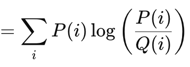
Where

• P is the probability that is forecast
• Q is the actual probability

Its outputs range from 0 which would indicate no divergence and up to infinity. These positive only values are a clear indicator of how far a forecast is from the ‘truth’. As shown in the formula above before this, the summation is only relevant when targeting a scalar output. The inbuilt vector implementation of this in MQL5 provides a vector output that is more suitable and needed in computing deltas and eventually gradients when performing back propagations. Kullback-Liebler Divergence is founded in information theory and has found some applications in reinforcement learning, given its dexterity, as well as in variational auto-encoders. Its cons though are asymmetry, sensitivity to zero values, and challenges in interpretation given the unbound nature of its output. The zero sensitivity is important because if one class is given a probability of zero the other has an infinite value automatically, but the asymmetry not only hampers the proper interpretation of the given probability, it makes transfer learning more difficult. (The probability of P given K is not inverse to that of K given P). The sums of the forward and reverse probabilities are not a predefined value. Sometimes it's infinity, sometimes it’s not.

This leads us to cosine similarity which, unlike the vector gap measures we have looked at this far, does consider direction. Its formula is given as follows:

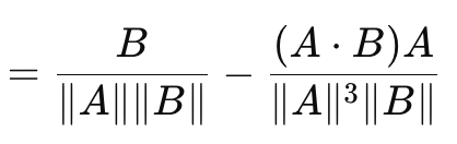
Where

• A.B is the dot product of two vectors
• ||A|| and ||B|| are their magnitudes or norms

The formula above is for the loss-gradient with respect to vector A. That with respect to vector B is a separate inverse formula and when summed to the cosine of A to B does not result in a fixed or arbitrary constant. To this end, cosine similarity is not a true metric since it does not satisfy the triangle of inequality. (The cosine similarity of A to B plus the cosine similarity of B to C is not always more than or equal to the cosine similarity from A to C). Its advantages are scale invariance since the value it provides is independent of the magnitude of the vectors in question, which can be important where direction and not magnitude is what is important. In addition, it is less compute intense than other methods, which is a key consideration when dealing with very deep networks or transformers or both! It has found high applicability for high dimensional data like text embeddings of large language models, where the inferred direction (meaning?) is a more relevant metric than the individual magnitudes of each vector value. Its cons are, it is not suitable for all tasks, especially in situations where the magnitude of vectors when training is important. Also, in the event that one of the vectors has a norm of zero (where all values are zero) then the cosine similarity would be undefined. Finally, it's already mentioned inability to be a metric from not fulfilling the inequality triangle rule. Examples of where this is crucial may be a bit wonkish, but they include: geometric deep learning, graph based neural networks, and contrastive loss from Siamese networks. In each of these use cases, magnitude is more important than direction. In applying the cosine similarity in MQL5 though, it is important to note it is the cosine proximity that is used and returned since this is more pertinent to machine learning. It is the distance equivalent of the angle’s cosine, and it is got by subtracting the cosine similarity from one.

The Poisson loss-gradient function is suitable for modelling countable or discrete data. It is like the loss functions mentioned above are implemented via the vector data-type’s in-built functions. Its formula is given by:

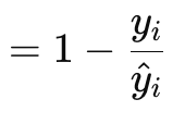
Where

• y is the target vector value (at index i)
• y^ is the forecast value

Gradient values are returned in vector format because this serve the back-propagation process much better. They are also first order derivatives of the original Poisson function scalar returning formula, which is:

Where

• representations much the gradient formula

The type of discrete data that traders could feed a neural network in this instance could include price bar candle types, or whether previous bars are bullish, bearish or flat.Its use cases though cover scenarios of counting data, so for instance a neural network that takes various candle price bar patterns that would be from recent history could be trained to return the number of a specific candle type that should be expected out of a standard sample of say 10 future price bars. Its coefficients are easy to interpret since they are log-rate ratios, and it aligns well with Poisson regression, meaning post training analysis can be easily done with the Poisson regression. It also ensures count forecasts are always positive (non-negative). It’s not, so good traits include variance assumption, where it is always assumed that the mean and variance have the same or almost similar values. If this is clearly not the case, then the loss function will not perform well. It is sensitive to outliers especially those with high counts in input data, the use of the natural logarithm does present a potential to yield NaN or invalid results. In addition, its application is restricted to positive countable data, meaning one would not use it in cases where continuous negative forecasts are necessary, such as when forecasting price changes.

Huber gradient-loss function concludes our sampling of what MQL5 has to offer within the vector data type. There are other classes we have not looked at like: logarithm of hyperbolic cosine, categorical hinge, squared hinge, hinge, mean-squared logarithmic error, and mean absolute percentage error. These are not critical to whether a neural network is a regressor or classifier, which forms part of our focus, and so we skimp-over them. Huber loss, though, is given by the formula:

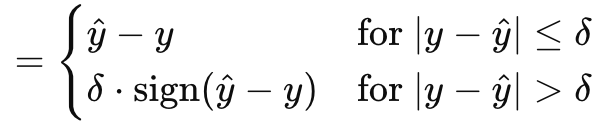
Where

• y^ is the forecast value
• y is the target
• Delta is a loss input value at which the relationship changes from linear to quadratic

The gradient, like the original Huber-loss, can be computed in one of two ways, depending on how the true or target value compares with the forecast. It is a part linear and part quadratic function that is a mapping of the difference between target values and forecast values as the input parameters are adjusted. It is predominant in robust regression since it combines the best of MAE and MSE and is less sensitive to outliers while being more stable than MAE for small errors. By being wholly differentiable it is ideal for gradient descent, and it is adaptable thanks to delta where a smaller delta has it acting like MAE while larger deltas have it more like MSE. This allows control over the robustness vs sensitivity trade off. On the cons side though Huber-loss is relatively more complex not only is its formula piece-wise as shown above the computation and determining of the ideal delta is often an onerous exercise. To this end, the MQL5 implementation, which I think is based on a standard matrix and vector library that I have failed to reference, does not disclose how its delta value is computed for the Huber-loss and Huber-loss gradient inbuilt functions. Though it can be paired with a variety of activation functions, the linear activation is often recommended as the more suitable.

Loss Functions for Regression Models

So, which of these loss algorithms would therefore be a best fit for regression networks? The answer, MSE, MAE, and Huber-Loss. Here’s why. Regression networks are characterized by their goal of forecasting continuous numerical values rather than categorical labels or discrete data. This implies the output layer of these networks typically produces real-valued numbers that can span a wide range. The nature of regression tasks requires minimizing the need to measure out wide-ranging deviations between predicted and true values, in their optimization, unlike in classification networks where the outputs that need to be enumerated are often few and known in number beforehand.

This therefore leads us to MSE. As observed above it does have large quadratic penalties for large errors which implies off the bat that it guides the gradient descent and optimization towards narrower deviations which is important for regression networks to run efficiently. Also, the smoothness and ease in differentiation makes it a natural fit for the continuous data handled by regression networks.

Regression networks are also susceptible to outliers a lot, and this therefore necessitates a loss function that is a bit robust in handling this. Enter MAE. Unlike MSE that imposes quadratic penalties on its errors, MAE imposes linear penalties and this make it less sensitive to outliers when compared to MSE. In addition, its error measure is a robust average error, which can be useful in noisy data.

Finally, regression networks in addition to the above, it is argued, need a balance or trade-off mechanism between sensitivity to small errors and robustness. These are two properties that the Huber-loss function provides and furthermore they offer smoothness which helps in differentiation throughout the optimization process.

With all three ‘ideal’ loss functions zeroed in, what would be the ideal palette of activation functions to consider when using them in a regression network? Officially, the recommendations are for linear activation and identity activation, with the latter implying the network outputs are preserved in their magnitude in order to capture as much of the data variability as possible. The main arguments for these two are the unbound nature of their outputs ensures no loss in data through the network feed forwards processes and training. Personally, I am a believer in bounded outputs, so I would rather opt for Soft-Sign and TANH as these capture both negative and positive real numbers, but they are bound to -1.0 to +1.0. I think bounded outputs are important because they avoid the problems with exploding and vanishing gradients during back propagation that are a major source of headache.

Loss Functions for Classification Models

What about classification neural networks? How would the choice for loss & activation functions fare? Well the process in arriving at our choices here does not differ much, we essentially look at the network key characteristics and they guide our choices.

Classification networks are purposed to forecast discrete class labels from a pool of predefined possible categories. These networks output probabilities indicating the likelihood of each class, with the chief goal being to maximize accuracy of these predictions through minimizing the loss. The choice of loss function therefore plays a key role in training the network to distinguish and identify the classes. Based off of these key features, consensus is for Categorical Cross Entropy and Binary Cross Entropy as being the two key loss functions best suited for classification networks out of the enumeration provided by MQL5.

BCE classifies out of two possible categories, however the number of predictions to be made can often be more than two and the size of this batch determines the norm of the gradient vector. So, the value at each index of the gradient vector would be a partial derivative of the BCE loss function as highlighted above in the shared formula and these values would be used in back-propagation. However, the network output values would be probabilities to the positive class as mentioned above, and they would be for each projected value in the output vector.

BCE is suitable for classification networks because the probabilities are easily interpretable since they point to the positive class. It is sensitive to the various probabilities of each output value, since it focuses on maximizing the log-likelihood of the correct classes from the batch. Because it can be differentiated not as a constant, but a variable, this greatly facilitates a smooth and efficient gradient computation in back propagation.

CCE expands BCE by allowing classifying more than 2 categories, and the norm or size of the output vector is always the number of classes for which a probability is given for each. This is unlike BCE where we could be making forecasts for up to say 5 values and all values for each are either true or false. With CCE, the output size is prefixed to match the class number. One-hot-encoding as mentioned earlier on is useful in normalizing the target vectors before the gaps to the forecast are measured.

The ideal form of activation to pair with this, it follows, would be any function that outbounds in the range 0.0 to +1.0. This includes Soft-Max, Sigmoid, and Hard Sigmoid.

Testing

We perform 2 sets of tests therefore, one for a regressive MLP, and one for a classifier. The purpose of this testing is to demonstrate implementation in MQL5 and Expert-Advisor-form of the loss-function and activation ideas discussed in this article. These presented test results are not a vindication to deploy and use the attached code on any live accounts but rather they are an invitation to the reader to perform his own diligence with testing on his Broker’s real-tick data over extended periods, should he deem the trade system(s) suitable. Deployment to live settings, as always, should be only ideal after cross validation or forward walk testing that yields satisfactory results has been performed.

So, we’ll be testing GBPCHF on the daily time frame over last year, 2023. To get a regressive network we’ll reference the ‘Cmlp’ class we introduced in the last article and since our input data will be price change percentages (not points) we can test with TANH activation and the Huber loss function to see how tradeable our system could be. The custom signal long and short conditions are implemented in MQL5 as follows:

//+------------------------------------------------------------------+
//| "Voting" that price will grow.                                   |
//+------------------------------------------------------------------+
int CSignalRegr::LongCondition(void)
{  int result = 0;
   vector _out;
   GetOutput(_out);
   m_close.Refresh(-1);
   if(_out[0] > 0.0)
   {  result = int(round(100.0*(fabs(_out[0])/(fabs(_out[0])+fabs(m_close.GetData(StartIndex()) - m_close.GetData(StartIndex()+1))))));
   }
//printf(__FUNCSIG__ + " output is: %.5f,  and result is: %i", _out[0],  result);return(0);
   return(result);
}
//+------------------------------------------------------------------+
//| "Voting" that price will fall.                                   |
//+------------------------------------------------------------------+
int CSignalRegr::ShortCondition(void)
{  int result = 0;
   vector _out;
   GetOutput(_out);
   m_close.Refresh(-1);
   if(_out[0] < 0.0)
   {  result = int(round(100.0*(fabs(_out[0])/(fabs(_out[0])+fabs(m_close.GetData(StartIndex()) - m_close.GetData(StartIndex()+1))))));
   }
//printf(__FUNCSIG__ + " output is: %.5f,  and result is: %i", _out[0],  result);return(0);
   return(result);
}

We also do simultaneous testing of the Expert on history data with training of the network, both on each new price bar. This is another key decision that can be changed easily where training is performed once every 6 months or another pre-determined longer period to avoid over-fitting the network to short-term action. This regressor network is in a 4-7-1 3-layer sizing (where the numbers represent layer sizes) implying 4 recent price changes serve as inputs and the single output is the next price change.

Performing test runs on GBPCHF for the year 2023 on the daily does give us the following report:

For the classifier network we still use the ‘Cmlp’ class as our base and our input data will be the classifications of the past 3 price points. This will feed into a 3-6-3 simple MLP network, also only 3-layers, where since we are looking at 3 possible classifications and our loss function is CCE, the final output layer should also be sized 3 so that it serves as a probability distribution. The generation of long and short conditions is implemented in MQL5 as follows:

//+------------------------------------------------------------------+
//| "Voting" that price will grow.                                   |
//+------------------------------------------------------------------+
int CSignalClas::LongCondition(void)
{  int result = 0;
   vector _out;
   GetOutput(_out);
   m_close.Refresh(-1);
   if(_out[2] > _out[1] && _out[2] > _out[0])
   {  result = int(round(100.0 * _out[2]));
   }
//printf(__FUNCSIG__ + " output is: %.5f,  and result is: %i", _out[2],  result);return(0);
   return(result);
}
//+------------------------------------------------------------------+
//| "Voting" that price will fall.                                   |
//+------------------------------------------------------------------+
int CSignalClas::ShortCondition(void)
{  int result = 0;
   vector _out;
   GetOutput(_out);
   m_close.Refresh(-1);
   if(_out[0] > _out[1] && _out[0] > _out[2])
   {  result = int(round(100.0 * _out[0]));
   }
//printf(__FUNCSIG__ + " output is: %.5f,  and result is: %i", _out[0],  result);return(0);
   return(result);
}

Similar test runs for the classifier Expert Advisor does give us the following results:

Attached code is used via wizard assembly to generate Expert Advisors, for which there are guides here and here.

Conclusion

To sum up, we have gone through the itinerary of possible loss functions available within MQL5 when developing machine learning algorithms such as neural networks. There is a very long list that ironically is not even exhaustive, however we have emphasized a few key ones that work well with particular activation functions that we covered in previous articles, with the emphasis being on avoiding exploding/ vanishing gradients and efficiency. A lot of available loss functions would not necessarily be suitable for the typical regression and classifier networks not just because their outputs are unbound, but because they do not address the key characteristic requirements of these networks as we have highlighted which is why the loss functions considered were a smaller number of what is available.