
MQL5 Wizard Techniques you should know (Part 32): Regularization
Introduction
Regularization is another facet of machine learning algorithms that brings some sensitivity to the performance of neural networks. In the process of a network, there is often a tendency to over assign weighting to some parameters at the expense of others. This ‘biasing’ towards particular parameters (network weights) can come to hinder the network’s performance when testing is performed on out of sample data. This is why regularization was developed.
It essentially acts as a mechanism that slows down the convergence process by increasing (or penalizing) the result of the loss function in proportion to the magnitude of weights used at each layer junction. This is often done either by: Early-Stopping, Lasso, Ridge, Elastic-Net, or Drop-Out. Each of these formats is a little different, and we will not consider all the types, but we will instead dwell on Lasso, Ridge and Drop-Out.
We consider the benefits and use of regularization within the context of having a proper or synced pairing with activation and loss functions. The proper selection and pairing of these do at a minimum prevent the problems of exploding/ vanishing gradients which is why this author in the recent articles (of these series) has been a proponent for using sigmoid & soft-max activation together with Binary-Cross Entropy or Categorical Cross Entropy loss functions when handling classifier networks. Conversely, TANH of soft-sign activation when paired with MSE or MAE or Huber loss functions could be suitable when dealing with regressor neural networks.
We also emphasized the importance of pairing these select activation functions with appropriate range-bound batch normalization algorithms in a related past article, however the loss function is unbound. This means the additional term to the loss function (the regularization) is not necessarily bound to be paired to an activation function or batch-normalization function that is bound in an ideal range (-1 to +1 for regressors, and 0 to 1 for classifiers).
None-the-less, the regularization type selected needs to be considerate of whether the network is a regressor or a classifier, here’s why. If we were to use L1 Lasso for instance, by penalizing with just the absolute value of the weights, the training process tends to reduce a lot of the weights in the network layers to zero while leaving only the critical ones at an acceptable small non-zero values. This inherently creates sparsity amongst the output, a situation that augers well with classifier networks whose feature probabilities are being forecast. This is especially relevant in situations where within the forecast feature probabilities only a few features are expected to be important.
Conversely, in regressor networks where often the final output layer has a size of 1 (unlike classification network probabilities for example), the contribution of the various weights is often expected to be ‘more democratic’. And to achieve this the L2, or Ridge regularizer is better suited since it is weighted towards the square of the weights that leads to a more even contribution across layer weights towards the final output. The drop-out regularization could be an alternative to regularizing classifier networks, as it too does introduce some sparsity to the output results due to the random nullifying of some weights. We share the code for this in the attachments below, however our testing focuses on L1 and L2.
Regularization in Neural Networks
The two formats of regularization we are testing out below do penalize the loss function in proportion to the network weight's magnitude. This ‘magnitude’ is computed through a Norm function, which in our case is offered in quite a few varieties. Strictly speaking, though, this norm ought to be the magnitude sum of all the matrix values. This absolute value sum could easily be realized in MQL5 as follows:
//+------------------------------------------------------------------+
//| Typical Norm function                                            |
//+------------------------------------------------------------------+
double Norm(matrix &M)
{  double _norm = 0.0;
   for(int i = 0; i < int(M.Rows()); i++)
   {  for(int ii = 0; ii < int(M.Cols()); ii++)
      {  _norm += M[i][ii];
      }
   }
   return(_norm);
}
However, we are dipping our toes into matrix norms (thanks to the various functions available within the matrix data type). The matrix norms unlike the simple absolute are not as strange a fit, as it might initially seem, because it is argued they introduce structural awareness to the regularization weighting process. In addition, they allow control over certain desired network properties like smoothness in regressor networks while still offering flexibility to fine tune desired sparsity in classifier network outputs. So, the consideration of these extra properties, that often seem nuanced, in evaluating the weights matrices for regularization is what we will apply in our test results below. To be clear, we are considering up to nine different matrix norms for each of the 2 regularization approaches we’ll test for a regressor and classifier network.
In the last article where we focused on the loss function, we had two network types, a regressor and a classifier. We will stick with those formats in illustrating regularization for this article as well.
L1 Regularization (Lasso)
Lasso (or L1) regularization involves penalizing the loss function in proportion to the absolute weights’ value or weights’ matrix norms, as discussed above. This is formally defined by the equation below:
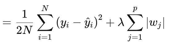
Where:
- N is the number of data points.
- p is the total number of layers for which there are weights matrices
- yi is the target (or label) value for the ith data point.
- y^i is the predicted value for the ith data point.
- wj are the coefficients (weights) of the model.
§λ is the regularization parameter that controls the strength of the regularization. A larger λ increases the penalty for large weights, promoting sparsity. Its optimal range can be 10-4to 10-1for soft-max or sigmoid activation networks, or 10-5to 10-2for soft-sign or TANH networks.
Put another way, the regularization value consists of the MSE the difference between the forecast values and the actual values (left side), plus the weights’ norm sum across all layers. We implement this in MQL5 as follows:
//+------------------------------------------------------------------+
//| Regularize Term Function                                         |
//+------------------------------------------------------------------+
vector Cmlp::RegularizeTerm(vector &Label, double Lambda)
{  vector _regularized;
   _regularized.Init(Label.Size());
   double _term = 0.0;
   double _mse = output.Loss(Label, LOSS_MSE);
   double _weights_norm = WeightsNorm();
   if(THIS.regularization == REGULARIZE_L1)
   {  _term = _mse + (Lambda * _weights_norm);
   }

        ....

   _regularized.Fill(_term);
   return(_regularized);
}
The output is a scalar value, not a vector and this contrasts a lot with what we have been dealing with as outputs of the loss function. Because when we need to define our update deltas which then help us set the update gradients in doing a back propagation, the loss is quantified as a vector. This vector helps feed into the delta vectors, which in turn update the gradient matrices. In order to maintain this, we create a vector that is filled with replicated values of the regularization value and use this as the output. This standard vector value then gets added to all the loss values in the loss vector, as defined by the loss function in use. This would be implemented as follows:
//+------------------------------------------------------------------+
//| BACKWARD PROPAGATION OF THE MULTI-LAYER-PERCEPTRON.              |
//+------------------------------------------------------------------+
//|                                                                  |
//| -Extra Validation check of MLP architecture settings is performed|
//|  at run-time.                                                    |
//|  Chcecking of 'validation' parameter should ideally be performed |
//|  at class instance initialisation.                               |
//|                                                                  |
//| -Run-time Validation of learning rate, decay rates and epoch     |
//|  index is performed as these are optimisable inputs.             |
//+------------------------------------------------------------------+
void Cmlp::Backward(Slearning &Learning, int EpochIndex = 1)
{

....

//COMPUTE DELTAS
   vector _last, _last_derivative;
   _last.Init(inputs.Size());
   if(hidden_layers == 0)
   {  _last = weights[hidden_layers].MatMul(inputs);
   }
   else if(hidden_layers > 0)
   {  _last = weights[hidden_layers].MatMul(hidden_outputs[hidden_layers - 1]);
   }

   _last.Derivative(_last_derivative, THIS.activation);
   vector _last_loss = output.LossGradient(label, THIS.loss);
   _last_loss += RegularizeTerm(label, THIS.regularization_lambda);

   deltas[hidden_layers] = Hadamard(_last_loss, _last_derivative);

        ...

}
So, a uniform penalty gets applied across all the features/ classes of the output vector and perhaps this is why one could make the case for using matrix norms and not just their absolute value, since the norms consider the matrix structure in their calculations.
In computing the regularization term, a number of matrix norms options are available and while all of them are usable in determining the Lasso, not all are suitable. The Frobenius norm is better aligned with L2 since it directly over penalizes large weights without enforcing sparsity, which is at odds with Lasso that aims to have non-critical weights adjusted to zero. The nuclear norm is better suited for promoting low rank matrices that are relevant to matrix completion problems. It is not aligned with Lasso that promotes element-wise sparsity as opposed to rank-sparsity. The spectral norm is also used in controlling the maximum effect a matrix has on a vector and not ensuring sparsity.
While infinity norms can create a form of sparsity, they are less ideal for creating element-wise sparsity. The minus infinity norm focuses on minimizing the smallest row sums, and this does not align with the Lasso sparsity objective. The same can be said for minus P1 and minus P2, as they both seek to minimize the influence of small elements.
So, from this enumeration of nine norms, it turns out only the P1 norm works best with Lasso because they promote sparsity with the goal of element-wise sparsity. P2 the final norm of the nine is better suited for L2 or Ridge regularization. So just to recap, L1 regularization was mentioned above as ideal for classifier networks. This implies a Classifier-L1-P1 relationship that has few alternatives for the weight’s matrix norms function.
L2 Regularization (Ridge)
L2 or Ridge regularization is very similar to L1 in formula, with the obvious difference being the squaring of weights’ norms as opposed to using the raw value. This is given as:
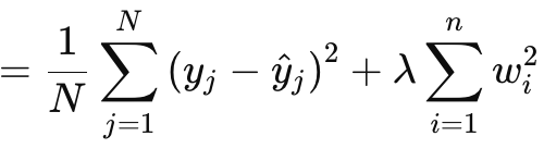
Where:
- λ is the regularization parameter that controls the strength of the penalty.
- w i are the weights or coefficients of the model.
- n is the number of layers with a preceding weights' matrix.
- N is the number of data points.
- y j is the actual target value.
- y^ j is the predicted value.
It, like L1, features an MSE and a term, which in this case is a sum of the squared weights. We implement this in MQL5 as follows:
//+------------------------------------------------------------------+
//| Regularize Term Function                                         |
//+------------------------------------------------------------------+
vector Cmlp::RegularizeTerm(vector &Label, double Lambda)
{  vector _regularized;
   _regularized.Init(Label.Size());
   double _term = 0.0;
   double _mse = output.Loss(Label, LOSS_MSE);
   double _weights_norm = WeightsNorm();

...

   else if(THIS.regularization == REGULARIZE_L2)
   {  _term = _mse + (Lambda * _weights_norm * _weights_norm);
   }


...

   _regularized.Fill(_term);
   return(_regularized);
}
The squaring of weights, as discussed above, does introduce smoothness to the regularization, which makes this approach an ideal candidate for regressor networks. In addition, the regularization is best handled by either Frobenius matrix norms or P2 norms. The two are actually the same, from what I can gather, with Frobenius being often used with matrices and P2 with vectors. Now from MQL5’s matrix norms functions, P2 can also be selected alongside Frobenius and the two return slightly different results. There is a post here on the differences between the two.
From all of this, therefore, the Regressor-L2-Frobenius pairing would be ideal with regressor neural networks.
Dropout Regularization
Finally, we have the drop-out regularization, which is markedly different from the two types we have looked at above. As a side note, the L1 and L2 can be combined in a weighted format to what is called the Elastic-Net, but that is left to the reader to try out and implement as all that would be required is an extra alpha parameter for proportioning the weights. Returning to the drop-out, it involves randomly choosing a neuron for omission, when training in the forward feed pass. This we implement in our MLP class as follows:
//+------------------------------------------------------------------+
//| FORWARD PROPAGATION THROUGH THE MULTI-LAYER-PERCEPTRON.          |
//+------------------------------------------------------------------+
//|                                                                  |
//| -Extra Validation check of MLP architecture settings is performed|
//|  at run-time.                                                    |
//|  Chcecking of 'validation' parameter should ideally be performed |
//|  at class instance initialisation.                               |
//|                                                                  |
//| -Input data is normalized if normalization type was selected at  |
//|  class instance initialisation.                                  |
//+------------------------------------------------------------------+
void Cmlp::Forward(bool Training = false)
{  if(!validated)
   {  printf(__FUNCSIG__ + " invalid network arch! ");
      return;
   }
//
   for(int h = 0; h <= hidden_layers; h++)
   {  vector _output;
      _output.Init(output.Size());

...

      if(Training && THIS.regularization == REGULARIZE_DROPOUT)
      {  int _drop = MathRand() % int(_output.Size());
         _output[_drop] = 0.0;
      }
      _output += biases[h];

...


   }
}
In the training and weight adjustment process, some weights can be adjusted to zero, so the fact we zeroized some of the output neuron values could be ineffective at achieving our intended result. Also, a manual multiplication that uses for loops during which we randomly omit neurons could have been a better approach at implementing the drop-out. It involves more coding, but the reader is welcome to attempt that.
We perform no testing with drop-out regularization because the benefits of this are usually only apparent on very deep & transformer stacked networks. For the purposes of this article we are only testing for L1 & L2, however the code for drop-out is attached and available for modification and testing on large networks.
Drop-out regularization is popular for a number of implementation reasons, and so let’s try to go through a few of them. Firstly, it prevents model over fitting by forcing the network to learn redundant representations. This ensures the network is not overly reliant on particular neurons or input features/ classes. This points to improved generalization. By randomly dropping neurons, the training process does create an ensemble of models from a single neural network. This improved generalization makes the network more robust at classifying unseen data, especially in complex, high dimensional data situations.
Furthermore, drop-out tends to make a network more resilient to noisy data by ensuring that no one neuron dominates the decision-making process. This is key not just with noisy or less reliable test data, but also in situations where the input data has a high degree of variance. In addition, it reduces neuron interdependency or encourages breaking neuron co-adaption. This encourages each neuron to learn independently, which makes the network more robust. Add to that, the use of drop-out in very deep and transformer stacked networks could not only introduce efficiency to the testing process (if the process manually drops neurons instead of the post-output vector approach we have adopted) but it also prevents the risk of over fitting given the large number of parameters involved.
It is applicable across various network formats like MLPs or CNNs and is scalable as well. When compared to L1 & L2, drop-out tends to lean more towards L1 as the dropping of neurons when testing leads to a sparser output results which are key in classifier networks. This is because most of the above-mentioned drop-out pros are pertinent to Classifier networks. These networks are often deeper than regressor networks, and these multitudes of parameters makes them prone to overfitting. Drop-out, as mentioned above, combats this by forcing the network to learn more general and robust features. Generalization is key in classifiers which drop-out enhances; noisy data can disproportionately affect them (when compared to regressor networks) and drop-out helps mitigate its effects. This and many of the already mentioned features above imply suitability for classifier networks because in general, but not always, classifier networks tend to have very few but large sized layers. They are very deep. On the other hand, regressor networks tend to have small sized but stacked layers. They lean more towards transformers. So, this perhaps is another key consideration that should be kept in mind not just when defining how a network is to be regularized but also in determining its overall layer number and sizes.
Test Results
As promised, as always, we perform tests with a wizard assembled Expert Advisor. For new readers, the attached code needs to be assembled into an Expert Advisor by following guidelines that are available here and here. We are testing on EURUSD this time, on the daily time frame for the yea 2023. As we performed in the last article, we are testing a regressor network and a classifier network.
As already argued in lead up articles to this one, classifier networks work best with soft-max or Sigmoid activations. In addition, as discussed above, they are more suited to work with Categorical Cross Entropy or Binary Cross Entropy loss functions and L1 regularization that specifically uses P1 matrix norms. Therefore, if we perform tests with these settings in place while placing pending orders on no stop-loss, we get the following results:

With the equity curve:

Conversely, for the regressor network if we perform tests using soft-sign activation and L2 Ridge regularization together with the Huber loss function, we do get the following results:

And the equity curve:

As a control to these results, one would need to train the network with reversed regularization options or no regularization at all. Test runs with identical settings with those used above for both the regressor and classifier networks but no regularization do produce the same results. This could imply regularization is not as critical as other factors like the loss function, activation functions and even the typical entry and closing thresholds of the Expert Advisor. However, a counter and perhaps credible argument could also be made that the benefits of regularization especially in the classifier network can best be appreciated with testing not just over longer periods that extend beyond a year but with very deep networks that feature a wider output class.
Conclusion
In conclusion, we have examined regularization as a key component of machine learning algorithms such neural networks by looking at its role in two particular settings. Classifier networks and Regressor networks. Classifier networks often, but not always, have very few layers but each of its layers is very deep. On the other hand, Regressor networks tend to have small sized layers, but they are stacked in multiples which ‘make-up’ for the lack of depth. While our test results indicate Expert Advisor, performance is not sensitive to regularization, based on the EURUSD runs on the daily time frame for 2023, more testing is warranted before such a drastic conclusion can be made. This is because besides the small test window, the networks used were on a very modest scale that is unlikely to reap the complete benefits of regularization.
Epilogue
I had intended to omit covering Elastic-Net regularization, however since the article is not too long I thought I could append it briefly here. The equation for Elastic-Net is as follows:
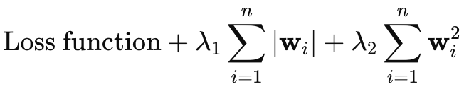
Where
- wi represents the individual weights of the model.
- λ1 controls the strength of the L1 penalty (Lasso), which encourages sparsity in the model by shrinking some weights to zero.
- λ2 controls the strength of the L2 penalty (Ridge), which encourages small weights but generally does not reduce them to zero.
To add the elastic-net regularization to our class, firstly we would have to modify the main enumeration to include it as follows:
//+------------------------------------------------------------------+
//| Regularization Type Enumerator                                   |
//+------------------------------------------------------------------+
enum Eregularize
{  REGULARIZE_NONE = -1,
   REGULARIZE_L1 = 1,
   REGULARIZE_L2 = 2,
   REGULARIZE_DROPOUT = 3,
   REGULARIZE_ELASTIC = 4
};
Then secondly, we would need to modify the ‘RegularizeTerm’ function to handle this Elastic-Net option by adding a 3rdif-clause and this we implement as follows:
//+------------------------------------------------------------------+
//| Regularize Term Function                                         |
//+------------------------------------------------------------------+
vector Cmlp::RegularizeTerm(vector &Label, double Lambda)
{  vector _regularized;
   _regularized.Init(Label.Size());
   double _term = 0.0;
   double _mse = output.Loss(Label, LOSS_MSE);
   double _weights_norm = WeightsNorm();

...


   else if(THIS.regularization == REGULARIZE_ELASTIC)
   {  _term =  _mse + (THIS.regularization_alpha * (Lambda * _weights_norm)) +
               ((1.0 - THIS.regularization_alpha) * (Lambda * _weights_norm * _weights_norm));
   }
   _regularized.Fill(_term);
   return(_regularized);
}
This clearly follows from the formula shared above, as it implements a weighted mean that uses an alpha value that is positive and does not exceed one. This would typically be optimized over the 0.0 to 1.0 range. From our code-implementation above, though, we are using a single matrix norm enumeration, which would prevent the capturing of the independent properties of L1 and L2. A walk around this is having two ‘_weight_norm’ variables each with their own matrix norm functions, but this would also mean the constructor struct should be modified to accommodate both. Alternatively, we could use the infinity norms as a compromise for both the regularization formats.
 Features of Custom Indicators Creation
 Features of Experts Advisors
- Free trading apps
- Over 8,000 signals for copying
- Economic news for exploring financial markets
You agree to website policy and terms of use