MQL5 Wizard Techniques you should know (Part 28): GANs Revisited with a Primer on Learning Rates

Introduction

We revisit a form of neural network we had considered in an earlier article by dwelling on one specific hyperparameter. The learning-rate. The Generative Adversarial Network is a neural network that operates in pairs, where one network is trained traditionally to discern the truth, while another is trained to discern the former’s projections from real occurrences. This duality does imply that the traditionally trained network (the former) is trying to fool the latter and this is true, however the two networks are on the ‘same team’ and the simultaneous training of both ultimately makes the generator network more useful to the trader. For this article, we dwell on the training process by focusing on the learning rate.

As always in these articles, the aim is to show-case signal classes, or trailing classes or money management classes that are not pre-installed in the library and yet could be compatible in some form to a trader’s existing strategies. The MQL5 wizard in particular allows the assembly and testing of this to be done seamlessly with minimal coding requirements for the common trade functions of an Expert Advisor. What can be taken from here is a custom class that can be tested independently as an assembled Expert Advisor or in parallel with other wizard classes, since the wizard assembly easily allows this. For anyone new to the wizard assembly process, these articles here and here do provide healthy introductions to the subject.

For this article therefore, within a simple Generative Adversarial Network (GAN), we will examine the significance, if any, learning-rates have on performance. ‘Performance’ itself is a very subjective term and strictly speaking testing should be carried out over periods much longer than we consider within these articles. So, for our purposes ‘performance’ will just be the total profit while taking into account, the recovery factor. There are several learning-rate types (or schedules) that we are going to consider, and an effort will be made to perform exhaustive testing on all, especially if they are clearly distinct from the pack.

The format of this article is going to differ somewhat from what we’ve been used to in prior articles. When presenting each learning rate format, its strategy testing reports will accompany it. This contrasts slightly with what we’ve had before, where the reports typically all came at the end of the article, prior to the conclusion. So, this is an exploratory format that keeps an open mind to the potential or not learning rates have on the performance of machine learning algorithms, or more specifically GANs. Because we are looking at multiple types and formats of learning rates it is important to have uniform testing metrics and that’s why we will use a single symbol, time frame and testing period throughout all the learning rate types.

Based on this, our symbol throughout will be EURJPY, the time frame will be the daily and the test period will be the year 2023. We are testing on a GAN and its default architecture is certainly a factor. There is always the argument that a more elaborate design in terms of number and size of each layer is paramount, however while those are all important considerations, our focus here is the learning rate. To that end, our GANs will relatively simple with just 3 layers that include one hidden layer. Overall sizing of each will be 5-8-1 from input towards output. The settings for these are indicated in the attached code and can easily be modified by the reader if he wishes to use an alternative setting.

To generate the long and short conditions, we are implementing all the different learning rate formats in the same way we did in this afore mentioned article that explored the use of GANs as a custom signal class in MQL5. That source code as always is attached however it is presented below for completeness:

//+------------------------------------------------------------------+
//| "Voting" that price will grow.                                   |
//+------------------------------------------------------------------+
int CSignalCGAN::LongCondition(void)
{  int result = 0;
   double _gen_out = 0.0;
   bool _dis_out = false;
   GetOutput(_gen_out, _dis_out);
   _gen_out *= 100.0;
   if(_dis_out && _gen_out > 50.0)
   {  result = int(_gen_out);
   }
   //printf(__FUNCSIG__ + " generator output is: %.5f, which is backed by discriminator as: %s", _gen_out, string(_dis_out));return(0);
   return(result);
}
//+------------------------------------------------------------------+
//| "Voting" that price will fall.                                   |
//+------------------------------------------------------------------+
int CSignalCGAN::ShortCondition(void)
{  int result = 0;
   double _gen_out = 0.0;
   bool _dis_out = false;
   GetOutput(_gen_out, _dis_out);
   _gen_out *= 100.0;
   if(_dis_out && _gen_out < 50.0)
   {  result = int(fabs(_gen_out));
   }
   //printf(__FUNCSIG__ + " generator output is: %.5f, which is backed by discriminator as: %s", _gen_out, string(_dis_out));return(0);
   return(result);
}

Fixed Learning Rate

To start things off, the fixed learning rate is probably what most new users of machine learning algorithms use, since it is the simplest. A standard measure by which the weights and biases of an algorithm get adjusted at each learning iteration, it does not change at all throughout the different training epochs.

The advantages of a fixed rate stem from its simplicity. It is very easy to implement since you have one floating point value to use throughout all the epochs and this also makes the training dynamics more predictable, something which helps in better understanding the whole process as well as debugging it. In addition, this breeds reproducibility. In many neural networks especially, those that are initialized with random weights, the results on a given test run, are not necessarily reproducible. In our case throughout all the different learning rate formats, we are using a standard initial weight of 0.1 and an initial bias of 0.01. By having such values fixed we are better positioned to reproduce the results from our test runs.

Also, a fixed learning rate brings stability in the early training process because the learning rate does not decrease, or fall off in the later stages as is the case with most of the other learning rate formats. Data that is encountered later on in the test runs is considered to a similar degree as the oldest data. This makes benchmarking and comparing easier in cases when you are fine-tuning a network for another hyperparameter that is not the learning rate. This could for instance be the initial weight used by the neural network. By having a fixed learning rate, such an optimization search can more quickly arrive at a meaningful result.

The main problem with a fixed learning rate is suboptimal convergence. There is a concern that when training, the gradient descent could get stuck at local minima and not converge optimally. This is particularly important before the ideal fixed learning rate has been established. Also, there is the argument of poor adaptation which follows a general consensus that as successive training epochs are encountered, the need ‘to learn’ does not remain the same. The general view is it decreases.

With these pros and cons, though, we do get the following picture when a test run is performed for the year 2023 for the pair EURJPY on the daily time frame:

Step Decay

Up next is the step decay learning rate, which is really a fixed learning rate with simply two extra parameters that govern how the initial fixed learning rate is reduced with each subsequent epoch. This is implemented as follows in MQL5:

      if(m_learning_type == LEARNING_STEP_DECAY)
      {  int _epoch_index = int(MathFloor((m_epochs - i) / m_decay_epoch_steps));
         _learning_rate = m_learning_rate * pow(m_decay_rate, _epoch_index);
      }

So, determining the learning rate at each epoch is a two-step process. First, we need to get the epoch index. This is simply an index that measures how far along we are through the epochs, during a training session. Its value is heavily influenced by a second input parameter, the ‘m_decay_epoch_steps’.Our for-loop is counting down, not up as is typically the case, so we subtract the current i value from the total number of epochs and then perform a Math-Floor division of this against this second input. The rounded integer result from this serves as an epoch index that we use in quantifying by how much we need to reduce the initial learning rate at the current epoch. If our step size (2^ndinput value) is 5, then we always wait and only reduce the learning rate after every 5 epochs. If the step size is 10, then the reduction is after 10 epochs, and so on.

The overall strategy of step decay is to gradually reduce this learning rate so as not to ‘overshoot’ the minimum and efficiently arrive at the optimal solution. It prides itself in providing a balance between fast initial learning and fine-tuning later on. It can help escape the local minima and saddle points in the loss landscape and often leads to better generalization through the learning rate reduction (unlike the fixed rate) and this could help in avoiding over-fitting.

If we do runs as above for EURJPY on the daily for the year 2023, we do get the following:

Exponential Decay

The exponential decay learning rate unlike the step decay rate is smoother in its reduction of the learning rate. Recall above we saw how the step decay learning rate only gets reduced when the epoch index increases or after a pre-defined number of epoch steps. With exponential decay, the reduction in learning rate is always occurring with each new epoch. This is represented by the formula below:

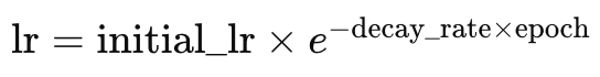
Where

• lr is the learning rate
• initial_lr is the initial learning rate
• e is Euler’s constant
• decay_rate and epoch represent their names respectively

This would be coded in MQL5 as follows:

      else if(m_learning_type == LEARNING_EXPONENTIAL_DECAY)
      {  _learning_rate = m_learning_rate * exp(-1.0 * m_decay_rate * (m_epochs - i + 1));
      }

The exponential decay is able to reduce the learning rate by multiplying it by a decay factor at each new epoch. This ensures a more gradual reduction in the learning rate when compared to the stepped approach above. Advantages of a gradual approach tend to fall more in line with general approaches at reducing the learning rate. These are already shared above with the step decay method. What exponential decay could provide that is missing with step decay, is the avoidance of sudden drops in the learning rate that can destabilize the training process.

If we perform test runs as above for EURJPY on the daily time frame for the year 2023, we do get the following results:

Even though the exponential decay allows a smoother and gradual reduction in the learning rate, by revising the learning rate at each epoch, not all reduction steps are the same size. At the onset of training, the reductions in the learning rate are significantly larger, and these values get reduced as the training progresses towards the last epochs.

Polynomial Decay

This, like the exponential decay also reduces the learning rate as training progresses. The main difference from exponential decay is that polynomial decay starts by reducing the learning rate slowly. The rate of reduction increases eventually as the training approaches the latter epochs of the process. This can be represented in an equation as follows:

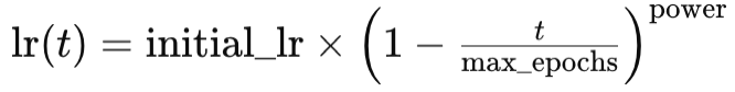
Where

• lr(t) is the learning rate at epoch t
• initial_lr is the initial learning rate
• t is the epoch’s index
• max_epochs and power represent their names respectively

The implementation would therefore be as follows:

      else if(m_learning_type == LEARNING_POLYNOMIAL_DECAY)
      {  _learning_rate = m_learning_rate * pow(1.0 - ((m_epochs - i) / m_epochs), m_polynomial_power);
      }

Polynomial decay introduces the ‘power’ input parameter to our signal class. All learning rate formats are being combined into a single signal class file, where the input parameters allow for the selection of a specific learning rate. This code file is attached at the bottom of the article. The polynomial power input is a constant exponent to a factor that we use to reduce the learning rate depending on the epoch, as shown in the formula above.

The polynomial decay like the exponential decay, and the step decay all reduce their learning rates. What could set the polynomial decay apart from this pack is, as mentioned above, the rapid reduction in the learning rate towards the end of training. This latter rapid reduction tends to allow for ‘fine-tuning’ of the training process in that the learning rate is kept as high as possible for as long as possible and only getting reduced when the epochs are being exhausted. This ‘fine-tuning’ is achieved by determining the optimal polynomial power over various training skits, and once this is determined, a more optimal learning process can be expected.

Advantages of polynomial decay are similar to what we’ve mentioned above with the other learning rate formats, primarily centring around the gradual reduction, which provides a smoother process on the whole. The fine-tuning of the learning rate as mentioned in addition to determining the ideal learning rates through the epochs, it also allows for the control of the amount of time the training process takes. A larger polynomial power can be understood to hasten the training process, while a low power should slow it down.

Test runs on EURJPY daily time frame over 2023 do give us the following results:

Inverse Time Decay

Inverse time also reduces the learning rate on a per-epoch basis by what is referred to as time-decay. Whereas above we considered rapid initial reduction in the learning rate with exponential decay versus slow reduction in the learning rate with polynomial decay, time decay allows for even slower reduction in the learning rate making it better suited than even the polynomial decay when handling very large training data sets.

The formula for inverse time is:

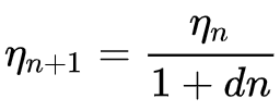
Where

• ηn+1 is the learning rate at epoch n + 1
• ηn is the prior learning rate at epoch n
• d is the decay rate
• and n is the epoch index.

We do implement this in MQL5 as follows:

      else if(m_learning_type == LEARNING_INVERSE_TIME_DECAY)
      {  _learning_rate = m_prior_learning_rate / (1.0 + (m_decay_rate * (m_epochs - i)));
         m_prior_learning_rate = _learning_rate;
      }

This algorithm is ideal for very large training data sets, given the way it really slows down the reduction in the learning rate. It shares most of the advantages already mentioned with the other learning rate formats. It is included here as a study sample to see how it would compare against these other learning rates when tested on the same symbol, time frame and test period. Full source is attached, so the user can make changes in order to perform more elaborate tests. If we do a test run though, following the settings we have been using this far, we get the following results:

Cosine Annealing

The cosine annealing rate scheduler also reduces the learning rate, gradually, towards a pre-set minimum by following a cosine function. The learning rate reduction objective is similar to the formats mentioned above, however with cosine annealing there is a target minimum, and the process keeps getting restarted whenever the minimum learning rate is hit until all epochs are exhausted.

The formula for this can be presented as follows:

Where

• lr(t) is the learning rate at epoch t
• initial_lr is the initial learning rate
• t is the epoch’s index
• T is the total number of epochs
• min_lr is the minimum learning rate

The implementation of this in MQL5 can be as follows:

      else if(m_learning_type == LEARNING_COSINE_ANNEALING)
      {  _learning_rate = m_min_learning_rate + (0.5 * (m_learning_rate - m_min_learning_rate) * (1.0 + MathCos(((m_epochs - i) * M_PI) / m_epochs)));
      }

Cosine annealing is better suited for large data sets, even more so than inverse time decay. This is because, whereas inverse time decay sufficiently postpones the large drops in the learning rate towards the last training epochs, cosine annealing allows a ‘reset’ of the learning by having it restored to its initial value once a preset minimum learning rate is hit. This is similar but different from another technique referred to as ‘warm restarts’ where at a preset training cycle the learning rate gets restored to its initial value.

Warm restarts would be suitable in very large training scenarios where batches/ cycles are used such that each batch gets split into epochs, as opposed to the single batch approach we have been considering this far in all the learning rate formats. When batches are used, the reset or restoring of the learning rate to its original value would be performed automatically at the end of a given batch.

Testing results with the single batch format for cosine annealing does give us the following report:

In addition, fine-tuning is also possible with cosine annealing since we have an additional input parameter of minimum learning rate. Depending on the value we assign to this rate, not only can we control the quality/ thoroughness of the training process, but we can also determine how long the training throughout all the epochs will last. So, depending on the size of the training data one is faced with, this can be hugely significant.

To this end, it is often argued that cosine annealing provides a balance between exploration and exploitation. Exploration being the search for the ideal learning rate, especially through the adjustment and fine-tuning of the minimum learning rate; while Exploitation is used to refer to harvesting the best network weights and biases while utilizing the best-known learning rates. This tends to lead to improved generalization of the model given the two-pronged optimization.

Cyclical Learning Rate

The cyclical learning rate, unlike the formats we have looked at this far, starts by increasing the learning rate before eventually reducing it back to the minimum. This happens in a cyclical pattern. Training therefore always starts with the minimum learning rate on each cycle. It is guided by the following formula:

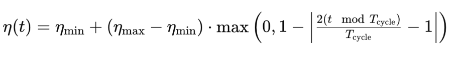
Where

• η(t) is the learning rate at epoch t
• ηmin is the minimum learning rate
• ηmax is the maximum learning rate
• Tcycle is the total number of epochs in a given batch or cycle (we are testing with single cycles only)
• (t modTcycle) is the remainder from dividing the number of epochs in a cycle by the epoch’s index. We multiply this value by 2

This we do implement in MQL5 as follows:

      else if(m_learning_type == LEARNING_CYCLICAL)
      {  double _x = fabs(((2.0 * fmod(m_epochs - i, m_epochs))/m_epochs) - 1.0);
         _learning_rate = m_min_learning_rate + ((m_learning_rate - m_min_learning_rate) * fmax(0.0, (1.0 - _x)));
      }

Performing test runs with this learning rate while sticking to the same symbol, time frame and test period settings we have been using above does give us these results:

There is another implementation of the cyclical learning rate called ‘triangular-2’ where once again initially the learning rate is increased after which it is reduced to the minimum. The difference here, though, from what we have looked at above is that the maximum learning rate value to which the rate is increased, keeps getting reduced with each cycle.

We will consider this learning rate format as well as additional formats that include the adaptive learning rate that by itself is relatively broad since it features different formats; warm restarts, and the single cycle rates for the next article.

Conclusion

To conclude, we have seen how the alteration of only the learning rate within a machine learning algorithm such as generative adversarial networks can yield a myriad of different results. Clearly, the learning rate is a very sensitive hyperparameter. The main of something that may seem jejune as a learning rate, is to arrive at the more concrete and sought-after network weights and biases and yet it is clear that the path chosen to arrive at these weights and biases, when testing within a fixed amount of time and resources, can vary significantly depending on the learning rate used.