Non-stationary processes and spurious regression

Contents

• Introduction
• Non-stationarity in regression analysis
• Testing statistical hypotheses about the regression model parameters
• Invalid specification of the regression model
• Conclusion

Introduction

As one of the sections of applied mathematical statistics, regression analysis is one of the most common methods of handling empirical data in the study of dependencies between random variables. While correlation analysis allows us to find out whether two random variables are related to each other, regression analysis gives an idea of what form this relationship might take. In regression analysis, a distinction is made between paired and multiple regression. In this study, I will use the well-known paired linear regression model for the sake of simplicity:

                                                Yt = b0 + b1Xt + et                                 (1)

• Yt - dependent variable (response);
• Xt - independent variable (or explanatory variable);
• b0, b1 model parameters; t - time (0,1,2,...n) n - number of observed data;
• et - random component, usually Gaussian white noise.

Here the index t is indicated in order to emphasize the fact that we are dealing with a time series, and that the sequence, in which the random variables are located, is important to us.

The task of regression analysis is:

• estimating the parameters of the selected regression model (in the linear case, using the ordinary least squares method)
• testing statistical hypotheses about the model parameters
• constructing confidence intervals for the obtained parameter estimates

If the analysis finds the model to be statistically significant, then it is considered to be suitable for use in predicting the dependent variable. But when applying regression analysis, especially to time series, we should always remember the limitation associated with the stationarity requirement imposed on the random sequences being studied. The requirement of stationarity assumes the invariance of the distribution function of a random variable over time and, consequently, the invariance of the mathematical expectation and variance of this random variable. Attempts to apply regression analysis to non-stationary processes can lead to false conclusions about the presence of a significant relationship between the variables under study. In this case, standard statistical tests, such as F-statistics and t-statistics, stop working and the risk of accepting a false dependence as true increases many times over.

Non-stationarity in regression analysis

In this article, I will use Monte Carlo simulation to show how spurious regression occurs when the stationarity assumption is violated, and also when the regression model is misspecified in the stationary case. For this I will use the standard MQL5 statistical library to generate random numbers and calculate critical values of the normal distribution and Student's distribution, as well as the graphics library to plot the obtained results. Calculating the regression model is greatly simplified by using the matrix algebra methods. For example, the equation for finding the regression model parameters using the least squares method in matrix form is written as:

(2) 

• X - matrix of values of independent variables;
• Y - dependent variable column vector;
• b - column vector of unknown parameters to be estimated from the sample.

In MQL5, the b vector (in our case of paired linear regression, it will consist of two elements - b0 and b1) can be found by calculating the pseudoinverse PInv() matrix of the X matrix and multiplying it by the Y vector:

pinv = x.PInv(); 

Coeff = pinv.MatMul(Y);  // vector of linear regression parameters using OLS

This is a shortened version of the calculation. We can calculate step by step as indicated in the equation:

xt = x.Transpose();

xtm = xt.MatMul(x);
inv = xtm.Inv();      
invt = inv.MatMul(xt);
Coeff_B = invt.MatMul(Y); // vector of regression parameters using OLS

The result will be the same.

For modeling purposes, we will need a random walk model as an example of a non-stationary process. We will build this model for both the dependent variable Y and the independent variable X. After that, construct a regression of Y on X and evaluate such an indicator as R-square (determination ratio), calculate the t-statistics and analyze the residuals of the regression model for correlation dependence.                                            

 Yt = Yt-1 + zt                           (3)

  Xt = Xt-1 + vt                           (4)

zt and vt  - two independently generated Gaussian "white noise" processes with zero mathematical expectation and N(0,1) unit variance;

Two possible trajectories of such a process are shown in Fig. 1

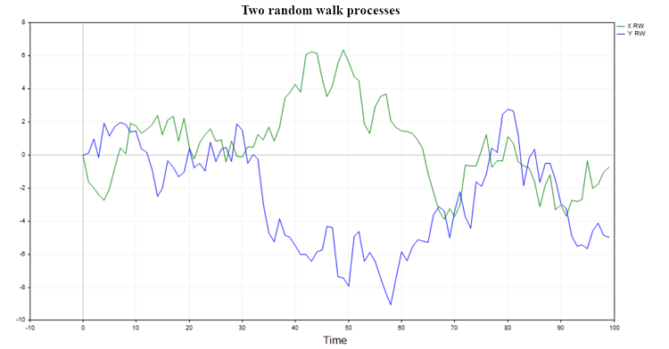
Fig. 1. Two random walks

Such processes have no memory and are not related to each other in any way, so it is natural to expect that the regression of one random walk on another should not give significant results and the hypothesis of a connection between two random walks will usually be rejected (with the exception of a small percentage of cases determined by the chosen significance level).

An example of one of the possible regressions is shown in Fig. 2:

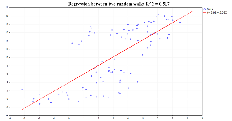
Fig. 2. Regression between two random walks, R2=0.517

The determination coefficient (R^2) is calculated using the equation: 

R^2 = 1 - SSE/TSS                              (5)

• SSE - sum of squared estimate of errors;
• RSS - sum of squares due to regression;
• TSS - total sum of squares = RSS+SSE;

The code for calculating all the main regression characteristics:

      pinv = x.PInv();
      Coeff = pinv.MatMul(Y);  // vector of linear regression parameters using OLS
      yRegression = x.MatMul(Coeff);  // y regression
      res = Y-yRegression;   //  regression residuals, y - y regression
      yMean = Y.Mean();
      reg_yMean = yRegression-yMean;  // y regression - mean y
      reg_yMeanT = reg_yMean.Transpose();
      RSS = reg_yMeanT.MatMul(reg_yMean);  // Sum( y regression - y mean )^2 , sum of squares due to regression
      resT = res.Transpose();
      SSE = resT.MatMul(res);  // Sum(y - regression y)^2
      TSS = RSS[0,0]+SSE[0,0];  // Total sum of squares
      RSquare = 1-SSE[0,0]/TSS;  // R-square determination ratio
      R2_data[s] = RSquare;

      Vres = SSE[0,0]/(T-2);           // residuals variance estimate
      SEb1 = MathSqrt(Vres/SX);        // estimate of the standard deviation of the b1 ratio deviation of the regression Y = b0 + b1*X;
      t_stat[s] = (Coeff[1,0]-0)/SEb1; // find the t-statistic for the b1 ratio under the hypothesis that b1 = 0;

R^2 values range from 0 to 1. In the case of paired linear regression, R^2 is equal to the square of the common correlation ratio between X and Y. When X does not affect Y, then R^2 is close to zero, and when the dependent variable Y is explained by the dependent variable X, then R^2 tends to one. In our case of regression of two independent random walks, it would be logical to expect that it would be distributed around zero. In order to check this, we will construct the distribution of R^2 by simulating 1000 pairs of random walks with 100 observations in each using the Monte Carlo method, with subsequent calculation of the R^2 ratio for each pair. As a result, we obtain the following distribution (Fig. 3):

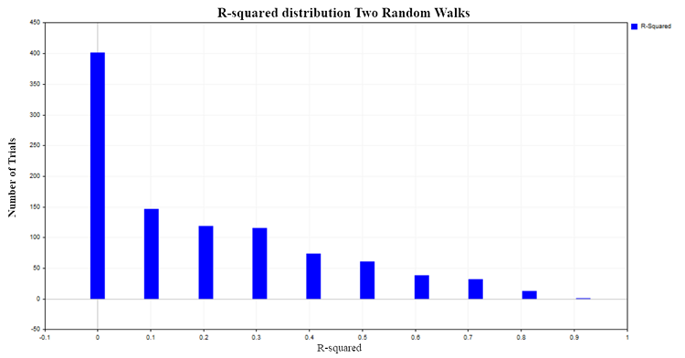
Fig. 3. R2 distribution for two random walks

In approximately 50% of cases, the determination ratio shows values greater than 0.2, indicating the presence of a relationship between quantities that are not related to each other. For comparison, let's obtain the R^2 distribution for two independent, but already stationary processes. A suitable model for such a process is the Gaussian white noise model.

                    Yt =  et                                   (6) 

 et  -  Gaussian white noise N(0,1)

Let's generate 1000 pairs of stationary random processes with 100 observations in each. As a result, obtain the expected distribution of R^2 around zero, Fig. 4:

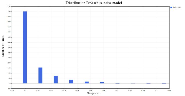
Fig. 4. R2 distribution, white noise model

Let's return to the two random walks and have a look at the behavior of t-statistic calculated to assess the significance of the parameters in our linear regression model.

Testing statistical hypotheses about the regression model parameters

The regression ratios calculated from the sample are themselves random variables and therefore there is a need to check the significance of these sample characteristics. When testing the significance of the b1 regression parameter, the null hypothesis (H0) is put forward that the explanatory variable X does not affect the dependent variable Y. In other words, H0(i) : b1 = 0 and the b1 parameter is not significantly different from zero. The alternative hypothesis (H1) states that the parameter b1 is significantly different from zero. That is, H1(i):b1 ≠ 0 and thus the predictor X influences the dependent variable Y.

To test this hypothesis, the t-statistic is used:

                                               t = bi /SEi                                      (7)

SEi - standard deviation of the bi estimated parameter 

This statistic has the Student's distribution ta/2 (n-p)  with (n-p) degrees of freedom.

• n - amount of data used for calculation in the regression model (in our case 100);
• p - number of estimated parameters (in our case of paired regression, there are 2);
• a - significance level (1,5,10%).

For our experiment, I chose the 5% significance level. Then if the t-statistics in absolute value exceed the critical value of the Student's distribution {|t| > t0.025 (98) =1.9844}, then we can conclude that the regression parameter b differs from zero1 and, as a consequence, there is a relationship between the explanatory variable X and the dependent variable Y. Since I chose the 5% significance level, we should expect only about 5% false rejections of the null hypothesis out of the total number of tests performed. But according to the simulation results, the t-statistic rejects the null hypothesis too often (falsely, since there is no dependence), approximately in 75% of cases (Fig. 5):

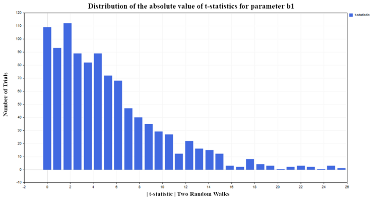
Fig.5. Distribution of the absolute value of the t-statistic for the b1 parameter

I would also like to note the following trend. The more observations in the sample, the greater the percentage of rejection of the null hypothesis. A seemingly paradoxical situation arises: the larger the sample, the more the X predictor affects the Y independent variable and the stronger the relationship between the variables. In fact, there is no paradox here, of course, but rather simply the application of regression analysis to processes it is not applicable to. We see that the standard t-statistic fails when regression is applied to the analysis of non-stationary time series. This situation is called spurious regression.

Invalid specification of the regression model

But non-stationarity is only one reason why standard statistical tests fail. They can be misleading even if the two series are stationary, but the specification of the regression model is violated. That is, if the wrong form of functional dependence between variables is chosen (linear instead of non-linear). Or if the model omits the X independent variable the Y variable actually depends on, and instead of it, a completely insignificant variable is mistakenly used. To clarify this, let's construct two independent X and Y stationary processes. As an example, I will use the first-order autoregressive model AR(1):

Yt = A*Yt-1 + zt                           (8)

 Xt = B*Xt-1 + vt                          (9)

• zt and vt - two independently generated Gaussian "white noise" processes with zero mathematical expectation and N(0,1) unit variance;
• A and B are parameters of the AR(1) model that should be strictly less than 1 in absolute value to satisfy the stationarity condition.

Let us again construct a regression of Y on X (for example, with AR(1) parameters A=0.5, B=0.5) under the same conditions as for the two random walks model (100 data in each process, number of tests 1000). As a result, we obtain the following t-statistics distribution for the b regression parameter b1 (Fig. 6):

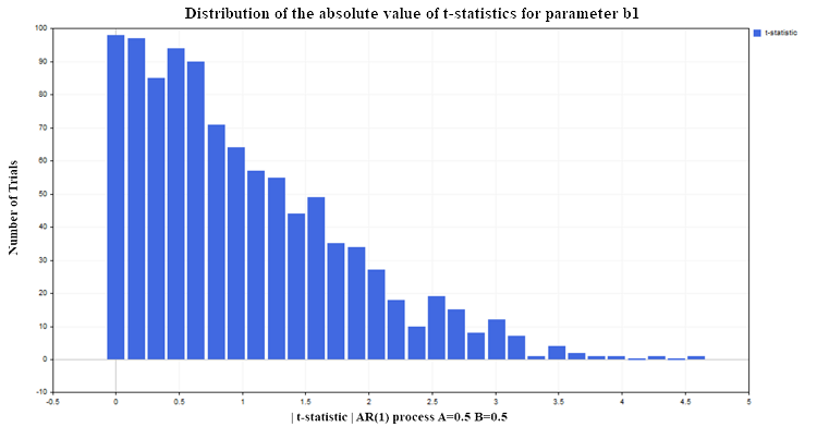
Fig. 6. Distribution of the absolute value of the t-statistic for the b1 parameter

As we can see, here the situation with the rejection of the null hypothesis is much better than in the non-stationary case. Only about 12-13% of false rejections with an acceptable level of 5% (the critical value of the Student's distribution for 98 degrees of freedom = 1.9844). For stationary processes, this percentage does not increase with an increase in the sample size, but remains at the same level. This time, the t-statistic fails not because the variables are non-stationary, which is fine, but because the regression model is incorrectly specified. Although the form of the dependence was chosen correctly (linear), we assumed that the Y variable does not depend on the lagged values of the same variable, but on the values of the X variable, which has no relation to the Y variable. If we leave the variable X in the regression model and add lagged values of Y to it, then the statistical properties of the regression parameters will improve and t-statistics will stop giving false conclusions more often than the established significance level (5% in our case). In practice, to understand that a regression model is spurious or incorrectly specified, one should turn to residual analysis. 

                                         Residuals =  Yt - Yreg_t                       (10)

• Yt - actual values of the Y dependent variable;
• Yreg_t  - calculated regression values

If there is significant auto correlation in the model residuals, this is a signal to consider the regression model to be misspecified or spurious. 

The code for calculating the auto correlation function (ACF) and 99% confidence intervals

////////////////////////// ACF calculation /////////////////////////////////////////

   avgres = res.Mean();  // mean of residuals
   ArrayResize(acov,K);
   ArrayResize(acf,K);
   ArrayResize(se,K);
   ArrayResize(se2,K);

   for(i=0; i<K; i++)
     {
      ArrayResize(c,T-i);
      for(j=0; j<T-i; j++)
        {
         c[j] = (res[j,0]-avgres)*(res[j+i,0]-avgres);
        }
      acov[i] = double(MathSum(c)/T);  // Auto covariance
      acf [i] = acov [i]/acov [0];  // Auto correlation
      se[i] =   MathQuantileNormal(0.995,0,1,err)/MathSqrt(T);    // 99% confidence intervals for ACF //
      se2[i] = -MathQuantileNormal(0.995,0,1,err)/MathSqrt(T);
     }

Fig. 7 shows the graph of the auto correlation function (ACF) of the regression residuals for the two random walks model. Also shown are the boundaries of the 99% confidence region for the ACF calculated using the equation SE = MathQuantileNormal(0.995,0,1,err)/MathSqrt(T); T - number of observations in the regression model.

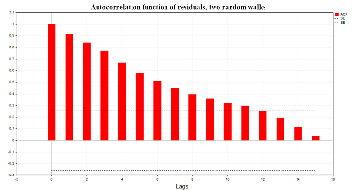
Fig. 7. Auto correlation function of residuals, two random walks

Fig. 8 shows the ACF chart of the regression residuals for a model of two AR(1) processes with parameters A=0.5, В=0.5

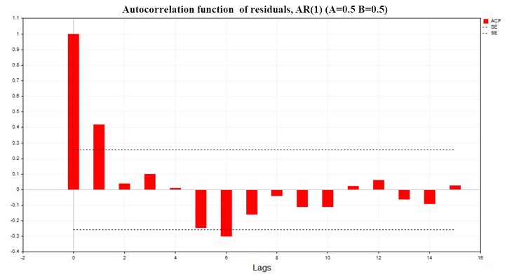
Fig. 8. Auto correlation function of residuals, AR(1)  A=0.5  B=0.5

As we can see from the graphs, there is significant auto correlation in the residuals of the regression models. Therefore, we are dealing with an incorrectly defined regression model or even a spurious regression. The Durbin-Watson (DW) criterion is also constructed based on the auto correlation function of the residuals. It is used to test the auto correlation of the residuals of a regression model with a lag of 1. 

                                            DW = 2*(1-ACF(1))                         (11)

In a spurious regression, this statistic is near zero.

Conclusion

The main issue I wanted to address in this article was understanding the limits of applicability of statistical methods, in particular regression analysis methods, as well as demonstrating the consequences of violating these limits. It is very easy to formally perform calculations, see "significant" statistics and draw the wrong conclusion about the presence of a connection between two random processes.

The conclusion that can be drawn from all of the above: 

• Before constructing a regression model, it is first necessary to test all variables in the model for stationarity.
• If some variable is non-stationary, it should be brought to a stationary form (usually by taking first differences) and then try to build a model with this modified variable.
• After building the model, it is necessary to examine the residuals for auto correlation dependence.
• If the values of the auto correlation function of the residuals do not go beyond the 99% confidence region, then we can proceed to assessing the significance of the parameters of the regression model using t-statistics.
• If it turns out to be significant, then we can begin to predict the Y dependent variable using the constructed model.

To reproduce all the above results, at the beginning of the script, select the values of the variable M = 1, 0 or 0.5, depending on which model you want to get the results for. After that, at the very bottom of the script, uncomment the block of code responsible for displaying certain statistics for each specific model. Also in the included Math.mqh file, comment out two strings of code for the function that calculates the empirical probability density function (MathProbabilityDensityEmpirical) to display frequencies on the graph

 5432  //  for(int i=0; i<count; i++)
 5433 //    pdf[i]*=coef;