
MQL5 Wizard Techniques you should know (Part 29): Continuation on Learning Rates with MLPs
Introduction
We revisit and conclude our look at the role different formats of learning rates have on Expert Advisor performance by examining the adaptive learning rates and the one cycle learning rate. The format for this article will follow the approach we had in the last article by having test reports at each learning rate format section rather than at the end of the article.
Before we jump in, we’d like to mention some of the other critical machine learning design considerations that can hugely sway the performance of a model. One of these is the batch normalization of the input data. I had touched on this in prior articles as to why it's significant, however our next article will squarely dwell on this. For now, though, when designing the mode and format of a network, batch normalization is considered in tandem with the activation algorithms to be employed by the model or network. Thus far we have been using soft plus activation which has the tendency of producing unbound results i.e. unlike the TANH or Sigmoid activations that produce outputs in the ranges -1.0 to +1.0 and 0.0 to 1.0 respectively, soft plus can quite often produce results that do not pass the valid test and thus render the training and forecasting process invalid.
As a pre-run to the next article, therefore, we are making some changes not just to the activation algorithms used by our networks but also the tested forex symbol. We are using the output-bound activation algorithm Sigmoid for all layer activations but more than that our test forex symbol pair will have its inputs (which in our case are still raw prices given we are not performing batch normalization) in the 0.0 to 1.0 range. There are not a lot of forex pairs that for our test period which is the year 2023, have their prices in this range; however, NZDUSD does, and so we will use it.
This does make comparing the performance results of the results in the previous article impractical, since the basis has changed. However, with this new network and activation algorithm and forex pair, the learning rate formats explored in the last article can still be tested by the reader in order to get a like for like comparison as one narrows down his preferred learning rate method. Also, the test results presented here and often in these articles in general are not from the best settings, nor are they meant to be. They are shown for exploratory purposes only, so it is always the reader's job to fine-tune the Expert Advisor's inputs for its optimum, not only with high-quality, historical data, but also preferably in forward testing after the strategy tester's period on demo accounts before it is deployed.
So, what is presented is only the potential. And to this end the learning rate has been shown to be a very sensitive metric on performance as is evident from the disparity of the test results we got in the last article. The adaptive learning rate is meant to address the problem of too many parameters determining the ideal learning rate for a model. Recall the learning rate itself is simply a means to the ideal network weights and biases, so the use of extra parameters like the polynomial power we saw in the last article, or minimum learning rate is meant to be avoided with these methods. To minimize the parametrization, in principle, adaptive learning generates the learning rate for each layer parameter by basing off of its training gradient. The impact of this is a situation where almost all parameters have their own learning rate, and yet the inputs provided to achieve this are minimal. Four formats of adaptive learning rates are common, namely: adaptive gradient, adaptive RMS, adaptive mean exponential, and adaptive delta. We’ll consider one at a time.
Adaptive Gradient Learning Rate
This is probably the simplest format amongst the adaptive learning rates, however it still adheres to the customized learning rate per parameter regime across all layers despite having a single input, the initial learning rate. The implementation of the learning rate on a per-parameter basis requires customizations that extend to our parent Expert class beyond the custom signal class, as we had in the last article’s learning rates. This is because the training gradients that serve as inputs determining the learning rate can only be accessed from within the parent network class interface. We can make changes to the class and make them public, but given the extra customization involved (where potentially each layer weight and bias could have its own learning rate) calling the backpropagation may cease to be as efficient as it ought to be. By working out each individual learning rate during the training process, the network is being primed to run almost as efficiently when a single learning rate is used across all parameters because the computed learning rate is applied immediately to the specific parameter rather than first developing a custom struct to house the new learning rates for all the parameters, then going through the iterative process of computing each learning rate separately, and then concluding with another iterative process of applying each individual learning rate. This would clearly not be more cumbersome to code, but it’s bound to be more compute intense. We are however making changes to the parent network class firstly by introducing two vector array parameters of ‘adaptive_gradients’ and ‘adaptive_deltas’ as shown in the new class interface below:
//+------------------------------------------------------------------+
//|                                                                  |
//+------------------------------------------------------------------+
enum ENUM_ADAPTIVE
{  ADAPTIVE_NONE = -1,
   ADAPTIVE_GRAD = 0,
   ADAPTIVE_RMS = 1,
   ADAPTIVE_ME = 2,
   ADAPTIVE_DELTA = 3,
};
//+------------------------------------------------------------------+
//|                                                                  |
//+------------------------------------------------------------------+
class Cmlp
{
protected:
   matrix            weights[];
   vector            biases[];

   vector            adaptive_gradients[];
   vector            adaptive_deltas[];

....

   bool              validated;

   void              AdaptiveGradientUpdate(double LearningRate, int LayerIndex, vector &Gradients, vector &Outputs);
   void              AdaptiveRMSUpdate(double DecayRate, double LearningRate, int LayerIndex, vector &Gradients, vector &Outputs);
   void              AdaptiveMEUpdate(double DecayRate, double LearningRate, int LayerIndex, vector &Gradients, vector &Outputs);
   void              AdaptiveDeltaUpdate(double DecayRate, double LearningRate, int LayerIndex, vector &Gradients, vector &Outputs);

public:

...

   void              Forward();
   void              Backward(double LearningRate = 0.1, ENUM_ADAPTIVE AdaptiveType = ADAPTIVE_NONE, double DecayRate = 0.9);

....

   void              ~Cmlp(void) { };
};
With these declared within the class interface, we then have to make significant changes to the backpropagation function, which we named ‘Backward’. Primarily, the changes involve adding inputs and checking these inputs to determine the appropriate type of learning rate to use. We only add two parameters to the ‘Backward’ function, namely ‘AdaptiveType’ and ‘DecayRate’. The adaptive type as the name suggests is one of the four adaptive learning rate types that would be provided if the adaptive learning rates are going to be used. Our network still leaves the option open of not using adaptive learning rates, which is why this parameter has a default value assigned of ‘ADAPTIVE_NONE’ which implies what its tag suggests. In addition, the next three formats of the adaptive learning rate we are going to look at below do require a decay rate so the 3rdand final input parameter to our back-propagation function will be this value and since the previous 2 parameters all have default values assigned, it follows that this one too is assigned a value.
Within this function the main changes are at the two ‘learning points’ i.e. where we update the output weights and biases as well as the scalable portion where we update the hidden weights and hidden biases of each hidden layer if the network has these. These update portions are separate because the inclusion of hidden layers is an option and not mandatory when constructing this network. It is scalable in that it will update all hidden layers at a go should they be present regardless of their number. So, the changes made from the old network back propagation are simply checking if adaptive learning is being used at each of these points. We have 4 adaptive learning rate types and all are presented below for completeness such that they are not repeated within the article after this. Our first point will now look as follows:
//+------------------------------------------------------------------+
//| Backward pass through the neural network to update weights       |
//| and biases using gradient descent                                |
//+------------------------------------------------------------------+
void Cmlp::Backward(double LearningRate = 0.1, ENUM_ADAPTIVE AdaptiveType = ADAPTIVE_NONE, double DecayRate = 0.9)
{  if(!validated)
   {  printf(__FUNCSIG__ + " invalid network settings! ");
      return;
   }
// Calculate output layer gradients
   vector _output_error = target - output;
   vector _output_gradients;
   _output_gradients.Init(output.Size());
   for (int i = 0; i < int(output.Size()); i++)
   {  _output_gradients[i] = _output_error[i] * ActivationDerivative(output[i]);
   }
// Update output layer weights and biases
   if(AdaptiveType == ADAPTIVE_NONE)
   {  for (int i = 0; i < int(output.Size()); i++)
      {  for (int j = 0; j < int(weights[hidden_layers].Cols()); j++)
         {  weights[hidden_layers][i][j] += LearningRate * _output_gradients[i] * hidden_outputs[hidden_layers - 1][j];
         }
         biases[hidden_layers][i] += LearningRate * _output_gradients[i];
      }
   }
// Adaptive updates
   else if(AdaptiveType != ADAPTIVE_NONE)
   {  if(AdaptiveType == ADAPTIVE_GRAD)
      {  AdaptiveGradientUpdate(LearningRate, hidden_layers, _output_gradients, hidden_outputs[hidden_layers - 1]);
      }
      else if(AdaptiveType == ADAPTIVE_RMS)
      {  AdaptiveRMSUpdate(DecayRate, LearningRate, hidden_layers, _output_gradients, hidden_outputs[hidden_layers - 1]);
      }
      else if(AdaptiveType == ADAPTIVE_ME)
      {  AdaptiveMEUpdate(DecayRate, LearningRate, hidden_layers, _output_gradients, hidden_outputs[hidden_layers - 1]);
      }
      else if(AdaptiveType == ADAPTIVE_DELTA)
      {  AdaptiveDeltaUpdate(DecayRate, LearningRate, hidden_layers, _output_gradients, hidden_outputs[hidden_layers - 1]);
      }
   }
// Calculate hidden layer gradients

...

}
Similarly, the changes to the hidden weights and biases updates are as follows:
//+------------------------------------------------------------------+
//| Backward pass through the neural network to update weights       |
//| and biases using gradient descent                                |
//+------------------------------------------------------------------+
void Cmlp::Backward(double LearningRate = 0.1, ENUM_ADAPTIVE AdaptiveType = ADAPTIVE_NONE, double DecayRate = 0.9)
{  if(!validated)
   {  printf(__FUNCSIG__ + " invalid network settings! ");
      return;
   }
// Calculate output layer gradients

...

// Calculate hidden layer gradients
   vector _hidden_gradients[];
   ArrayResize(_hidden_gradients, hidden_layers);
   for(int h = hidden_layers - 1; h >= 0;  h--)
   {  vector _hidden_target;
      _hidden_target.Init(hidden_outputs[h].Size());
      _hidden_target.Fill(0.0);
      _hidden_gradients[h].Init(hidden_outputs[h].Size());
      if(h == hidden_layers - 1)
      {  for(int j = 0; j < int(hidden_outputs[h].Size()); j++)
         {  double _sum = 0.0;
            for(int i = 0; i < int(target.Size()); i++)
            {  if(weights[h + 1][i][j] != 0.0)
               {  _sum += (target[i] / weights[h + 1][i][j]);
               }
            }
            _hidden_target[j] = ActivationDerivative(_sum - biases[h][j]);
         }
      }
      else if(h < hidden_layers - 1)
      {  for(int j = 0; j < int(hidden_outputs[h].Size()); j++)
         {  double _sum = 0.0;
            for(int i = 0; i < int(hidden_outputs[h + 1].Size()); i++)
            {  if(weights[h][i][j] != 0.0)
               {  _sum += (hidden_outputs[h + 1][i] / weights[h][i][j]);
               }
            }
            _hidden_target[j] = ActivationDerivative(_sum - biases[h][j]);
         }
      }
      vector _hidden_error = _hidden_target - hidden_outputs[h];
      for (int i = 0; i < int(_hidden_target.Size()); i++)
      {  _hidden_gradients[h][i] = _hidden_error[i] * ActivationDerivative(hidden_outputs[h][i]);
      }
   }
// Adaptive updates
   if(AdaptiveType != ADAPTIVE_NONE)
   {  for(int h = hidden_layers - 1; h >= 0;  h--)
      {  vector _outputs = inputs;
         if(h > 0)
         {  _outputs = hidden_outputs[h - 1];
         }
         if(AdaptiveType == ADAPTIVE_GRAD)
         {  AdaptiveGradientUpdate(LearningRate, h, _hidden_gradients[h], _outputs);
         }
         else if(AdaptiveType == ADAPTIVE_RMS)
         {  AdaptiveRMSUpdate(DecayRate, LearningRate, h, _hidden_gradients[h], _outputs);
         }
         else if(AdaptiveType == ADAPTIVE_ME)
         {  AdaptiveMEUpdate(DecayRate, LearningRate, h, _hidden_gradients[h], _outputs);
         }
         else if(AdaptiveType == ADAPTIVE_DELTA)
         {  AdaptiveDeltaUpdate(DecayRate, LearningRate, h, _hidden_gradients[h], _outputs);
         }
      }
   }
// Update hidden layer weights and biases
   else if(AdaptiveType == ADAPTIVE_NONE)
   {  for(int h = hidden_layers - 1; h >= 0;  h--)
      {  for (int i = 0; i < int(weights[h].Rows()); i++)
         {  for (int j = 0; j < int(weights[h].Cols()); j++)
            {  if(h == 0)
               {  weights[h][i][j] += LearningRate * _hidden_gradients[h][i] * inputs[j];
               }
               else if(h > 0)
               {  weights[h][i][j] += LearningRate * _hidden_gradients[h][i] * hidden_outputs[h - 1][j];
               }
            }
            biases[h][i] += LearningRate * _hidden_gradients[h][i];
         }
      }
   }
}
All the functions mentioned above in these changes will be highlighted in their respective sections. For the adaptive gradient update function, our implementation is as follows:
//+------------------------------------------------------------------+
// Adaptive Gradient Update function
//+------------------------------------------------------------------+
void Cmlp::AdaptiveGradientUpdate(double LearningRate, int LayerIndex, vector &Gradients, vector &Outputs)
{  for (int i = 0; i < int(weights[LayerIndex].Rows()); i++)
   {  adaptive_gradients[LayerIndex][i] += (Gradients[i] * Gradients[i]);
      double _learning_rate = LearningRate / (MathSqrt(adaptive_gradients[LayerIndex][i]) + __NON_ZERO);
      for (int j = 0; j < int(weights[LayerIndex].Cols()); j++)
      {  weights[LayerIndex][i][j] -= (_learning_rate * Gradients[i] * Outputs[j]);
      }
      //
      biases[LayerIndex][i] -= _learning_rate * Gradients[i];
   }
}
The added vector array of adaptive gradients accumulates squared values of gradients for each parameter at each layer. These squared values, which are specific to each parameter, then reduce the learning rate in various amounts depending on the parameter involved and its history of gradients throughout the training process. The squared gradients sum act as a denominator to the learning rate, so it can be understood that the larger the gradients, the smaller the learning rate.
We do perform some test runs with the adaptive gradient learning rates and some of our test results are as follows:
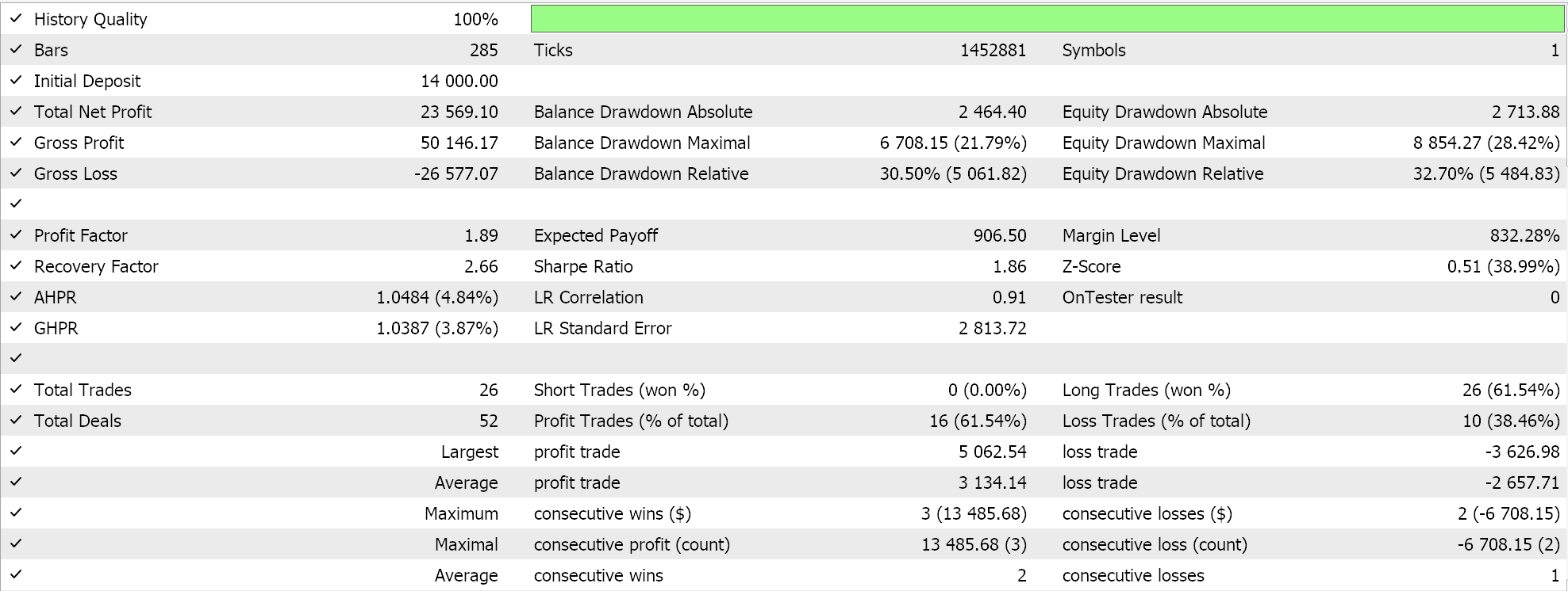
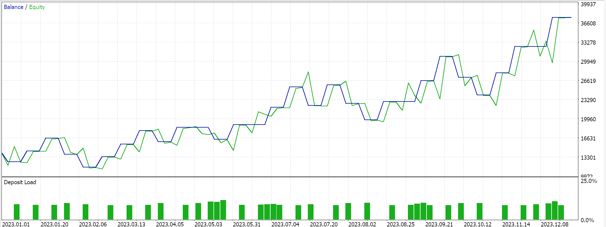
These test runs are made for the year 2023 on the daily time frame for the forex pair NZDUSD. The use of NZDUSD is for batch normalization purposes that we will cover in more detail for the next article. For now, though, as mentioned above, we are using Sigmoid activation that keeps its outputs in the 0.0 to 1.0 range and this bodes well for testing purposes when exploring ideal learning rates. Once each parameter has its own learning rate, the weights and biases get updated by the adaptive gradient update function, whose listing is already shared above.
Since our input data, of raw prices is within the 0.0 to 1.0 range, and we are activating by Sigmoid, our network outputs should also be in the 0.0 to 1.0 range. We are dealing with raw prices and since we are feeding our network historical price data and training it on sequential price data, we can expect our network to forecast the next close price. We are doing this all without batch normalization which is very risky as even though the output could be in the desired 0.0 to 1.0 range it can easily be skewed above the current bid price (or below it) which would give permanent buy or permanent sell signals. This is already apparent in our ‘ideal’ test results above. Now, I did make runs where both long and short positions were opened, but the lack of batch normalization is something to be wary of. In order to generate signals or condition values from our long and short condition functions in the custom signal class, we need to normalize the forecast price to be in the integer range of 0 to 100.
As always, there are a ton of ways this could be achieved, however in our case we simply compare the projected price to the array of input prices and come up with a percentile double value. We convert this percentile value into an integer in the expected 0 to 100, and we have an output condition. This normalization is only done in each of the long and short condition functions if the network’s forecast price is above the current bid or below the current bid price, respectively. The source code to this is shared below:
//+------------------------------------------------------------------+
//| "Voting" that price will grow.                                   |
//+------------------------------------------------------------------+
int CSignalCMLP::LongCondition(void)
{  int result = 0;
   double _mlp_output = 0.0;
   GetOutput(_mlp_output);
   m_symbol.Refresh();
   m_symbol.RefreshRates();
   if(_mlp_output > m_symbol.Bid())
   {  vector _scale;
      _scale.CopyRates(m_symbol.Name(), m_period, 8, 0, __MLP_INPUTS);
      result = int(round(100.0 * (fmin(_mlp_output, _scale.Max()) - _scale.Min()) / fmax(m_symbol.Point(), _scale.Max() - _scale.Min())));
   }
//printf(__FUNCSIG__ + " output is: %.5f, change is: %.5f, and result is: %i", _mlp_output, m_symbol.Bid()-_mlp_output, result);return(0);
   return(result);
}
//+------------------------------------------------------------------+
//| "Voting" that price will fall.                                   |
//+------------------------------------------------------------------+
int CSignalCMLP::ShortCondition(void)
{  int result = 0;
   double _mlp_output = 0.0;
   GetOutput(_mlp_output);
   m_symbol.Refresh();
   m_symbol.RefreshRates();
   if(_mlp_output < m_symbol.Bid())
   {  vector _scale;
      _scale.CopyRates(m_symbol.Name(), m_period, 8, 0, __MLP_INPUTS);
      result = int(round(100.0 * (fmin(_mlp_output, _scale.Max()) - _scale.Min()) / fmax(m_symbol.Point(), _scale.Max() - _scale.Min())));
   }
//printf(__FUNCSIG__ + " output is: %.5f, change is: %.5f, and result is: %i", _mlp_output, m_symbol.Bid()-_mlp_output, result);return(0);
   return(result);
}
The use of this code which is attached at the bottom of this article is by assembling an Expert Advisor via the MQL5 wizard. Guidance on doing that can be found here and here.
Adaptive RMS Learning Rate
The RMS prop adaptive learning rate introduces an extra parameter to manage the rapid drop-off in the learning rate that happens a lot when faced with large training gradients, as these do accumulate throughout the training process. This parameter is the decay rate, which we’ve already introduced above as one of the new extra input parameters to the modified back propagation function. In the previous article though we did use a decay rate in the step decay learning rate, exponential decay learning rate and inverse time decay learning rate, and it served a quasi-similar purpose. From our custom signal class, we have a solo input parameter named decay rate that serves all these purposes because in any training session only one learning rate format can be selected. So, the decay rate will serve the selected learning rate type.
To continue with adaptive learning rates though, the RMS-prop limits the accumulation of historic gradients, which can be a problem with the adaptive gradients since they slow down the learning significantly to a point where it effectively grinds to a halt. This is because of the inverse relationship between the historic gradients and the learning rate already mentioned above. RMS prop’s innovation, thanks to the decay factor, is to effectively slow down this drop in the learning rate and this is accomplished as follows:
//+------------------------------------------------------------------+
// Adaptive RMS Update function
//+------------------------------------------------------------------+
void Cmlp::AdaptiveRMSUpdate(double DecayRate, double LearningRate, int LayerIndex, vector &Gradients, vector &Outputs)
{  for (int i = 0; i < int(weights[LayerIndex].Rows()); i++)
   {  adaptive_gradients[LayerIndex][i] += (DecayRate * adaptive_gradients[LayerIndex][i]) + ((1.0 - DecayRate)*(Gradients[i] * Gradients[i]));
      double _learning_rate = LearningRate / (MathSqrt(adaptive_gradients[LayerIndex][i]) + __NON_ZERO);
      for (int j = 0; j < int(weights[LayerIndex].Cols()); j++)
      {  weights[LayerIndex][i][j] -= (_learning_rate * Gradients[i] * Outputs[j]);
      }
      biases[LayerIndex][i] -= _learning_rate * Gradients[i];
   }
}
Another problem with the adaptive gradient is that when dealing with non-stationary data and the underlying distribution & characteristics of the data change over time, and thus even through a training set, the accumulated gradients can become outdated and less relevant leading to suboptimal learning rates. RMS prop on the other hand sees to it that the more recent gradients are in play and therefore have greater influence on the learning rate. This makes the learning process more adaptable and arguably more useful in scenarios more pertinent to traders, like time series forecasting.
In addition, in cases where training is done on sparse data sets such as those outside our core competency of trading like in natural-language-processing or recommendation-systems adaptive gradients can excessively reduce gradients when reading infrequently used features or data points. RMS prop therefore allows a more balanced training process by maintaining the learning rate at a relatively higher level for longer periods, such that these networks (which traders could still find useful in certain situations) can have more optimal weights and biases.
Finally, adaptive gradients are very susceptible and sensitive to noisy data since in essence the gradient positively correlates to noise. So, in situations where the training data is not properly filtered for these outliers, rapid reductions in the learning rate would essentially imply the network would be learning more from the outliers and noise than the core or ideal data. RMS prop’s smoothing effect with the decay factor does mean that the learning rate can ‘survive’ the wild outliers and still continue to effectively contribute to the network weights and biases when the core or ideal data is eventually met in the training set.
We do perform some test runs with RMS prop adaptive learning and below is a sample of our test results:
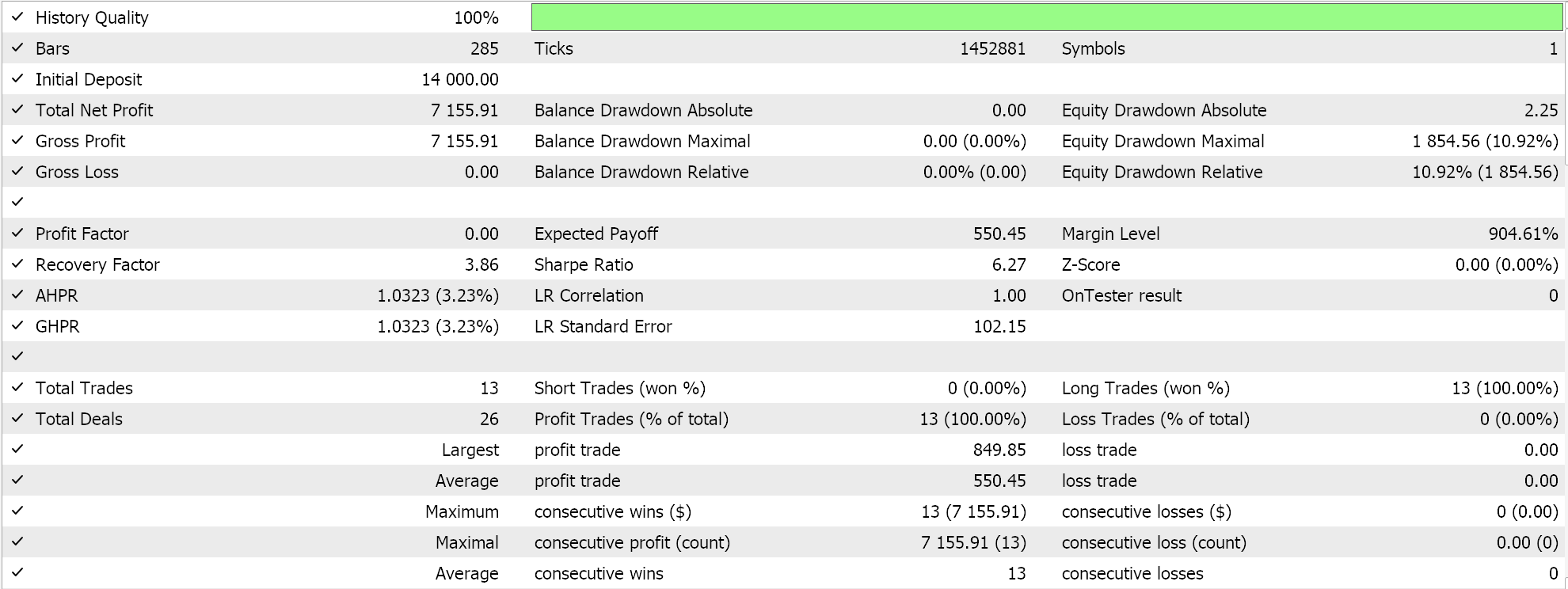
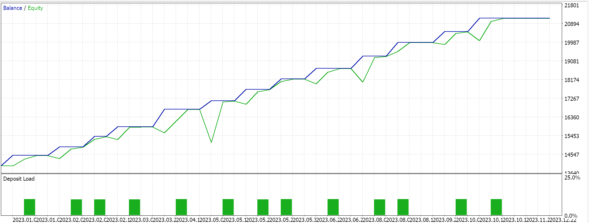
Because our network inputs are not batch normalized in line with the choice of activation function for this network (we are using Sigmoid vs Soft Max) our test results are skewed to only place long trades because the output forecast price was always above the current bid. There could be ways of normalizing the output price to give a balance between long and short positions, which our approach here has not considered, but I would prefer we start with proper batch normalization of the input data before we consider such approaches. This is therefore a problem we will tackle more effectively in the net article, as mentioned above.
Adaptive Moment Estimation (or Mean Exponential) Learning Rate
Adaptive Moment Estimation (aka ADAM) is another variant of adaptive learning rates that aims to make approaches like RMS above even smoother through a two-pronged consideration of both gradient mean and gradient variance (momentum). This is implemented in MQL5 as follows:
//+------------------------------------------------------------------+
// Adaptive Mean Exponential(ME) Update function
//+------------------------------------------------------------------+
void Cmlp::AdaptiveMEUpdate(double DecayRate, double LearningRate, int LayerIndex, vector &Gradients, vector &Outputs)
{  for (int i = 0; i < int(weights[LayerIndex].Rows()); i++)
   {  adaptive_gradients[LayerIndex][i] = (DecayRate * adaptive_gradients[LayerIndex][i]) + ((1.0 - DecayRate)*(Gradients[i] * Gradients[i]));
      double _learning_rate = LearningRate / (fabs(adaptive_gradients[LayerIndex][i]) + __NON_ZERO);
      for (int j = 0; j < int(weights[LayerIndex].Cols()); j++)
      {  weights[LayerIndex][i][j] -= (_learning_rate * Gradients[i] * Outputs[j]);
      }
      //
      biases[LayerIndex][i] -= _learning_rate * Gradients[i];
   }
}
We’ve just seen above how RMS prop learning rates are a step up from gradients rates in that they slow down the rate of reduction in the learning rate, and this can provide a number of advantages, some of which have been shared above. Well ADAM continues in this direction especially when faced in situations of high dimensional data. As the dimensions of handled data sets increases, so does the number of parameters in a gradient array. In situations such as these, that could be image and speech recognition, considering momentum in addition to the mean helps the learning rate adapt more sensitively to the data set than if only the mean was considered. Depending on one’s network design, such a high dimension scenario could be encountered in financial time series forecasting.
Relatively unstable and slow convergence when using only the mean of squared gradients makes RMS prop less reliable in noisy data than ADAM. The combination of both the squared means and variance provides a smoother, more robust, stable and faster handling of convergence. Also, sparse gradients in natural language processing and recommendation systems, although better handled by RMS prop than in adaptive gradient, are even managed better with ADAM thanks to momentum weighting in the learning rate. Furthermore, in situations where parameters change frequently such as when a new network is initialized with random weights and biases, RMS prop’s focus on recent gradient history can lead to overly conservative updates whereas ADAM’s momentum considerations allow it to still be better responsive even in these situations.
Finally, in dealing with non-stationary objectives where the objective function changes over time, RMS prop though assisted by a mean may still not adapt as well as ADAM. As an example of this, consider a situation where your network is modelled to forecast real estate prices, and it handles inputs or features like size of house, number of bedrooms, and location. The objective function we are using for our MLP network, during back propagation, is simply the vector difference between the target and the forecast, but typically this objective can take many forms such as mean squared error (MSE) where in this situation you would have the following formula:

Where:
- n is the number of houses in the data sample
- MSE is the mean-squared error
This would be a back-propagation error function whose result decreases over time as the network learns by appropriately updating its weights and biases, with lower MSE values signifying improved network performance. Now supposing the studied real estate market changes drastically such that the relationship between the network features (inputs) and the forecast prices changes significantly, where for instance a new metro is introduced in the region that is occupied by the examined real estate. This would certainly change the pricing model of the real estate property in that area, and this would make the objective function less useful in adapting to these changes. Revising the network by adding more pertinent features (input fields) could lead to a more optimal outcome as the weights and biases get updated. ADAM better manages this transition of revising and updating a network model through the addition of new features, since the weight update process factors in momentum.
Test results with ADAM do give us the following report:
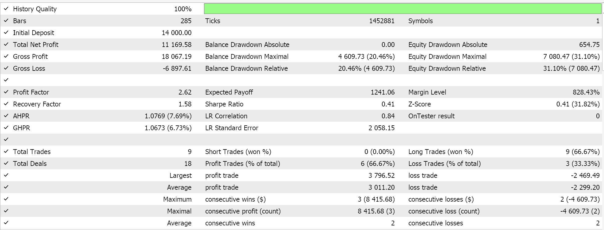
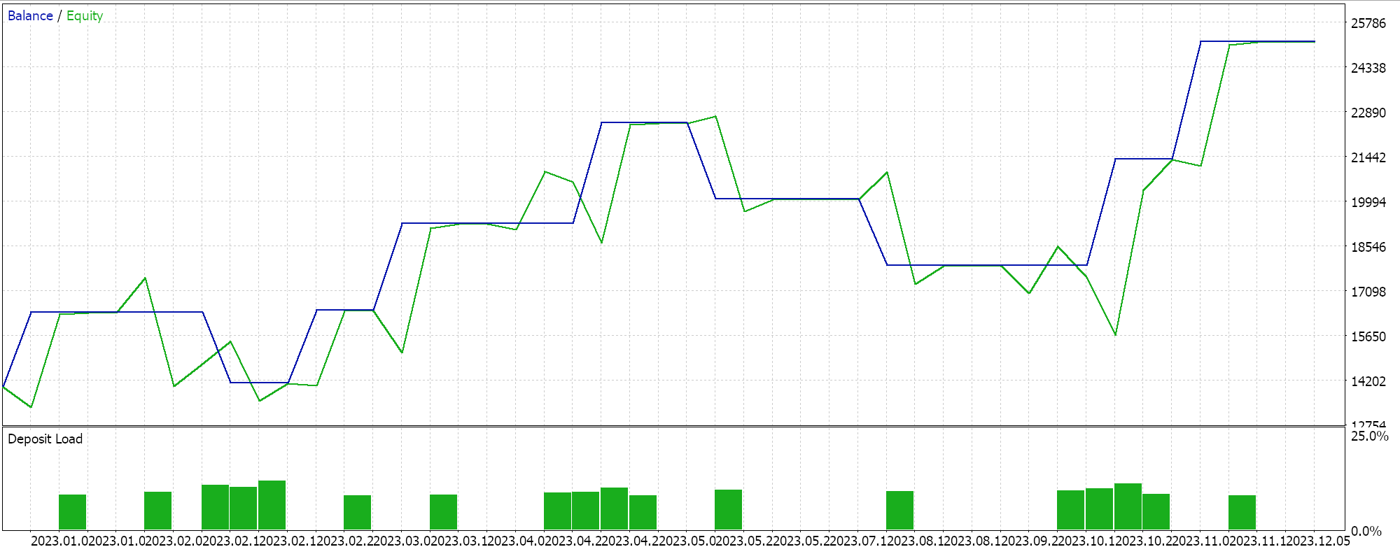
This is not from the best or ideal settings, but it only exhibits how the ADAM learning rate is applied in an MLP network. In the last article we had used a pair of GAN networks while here we are using something more rudimentary but still intuitive, the Multi-Layer-Perceptron with only three layers, in a 5-8-1 formation.
Adaptive Delta Learning Rate
Our final adaptive learning rate is the ADADELTA and even though it does not take on any new input parameters it furthers the effort of optimally adjusting the learning rate when training. The formula for this is relatively complicated, but in principle, besides taking into account a decayed accumulation of gradients, a decayed accumulation of weights is also considered. This is realized in MQL5 as follows:
//+------------------------------------------------------------------+
// Adaptive Delta Update function
//+------------------------------------------------------------------+
void Cmlp::AdaptiveDeltaUpdate(double DecayRate, double LearningRate, int LayerIndex, vector &Gradients, vector &Outputs)
{  for (int i = 0; i < int(weights[LayerIndex].Rows()); i++)
   {  adaptive_gradients[LayerIndex][i] = (DecayRate * adaptive_gradients[LayerIndex][i]) + ((1.0 - DecayRate)*(Gradients[i] * Gradients[i]));
      double _delta = (MathSqrt(adaptive_deltas[LayerIndex][i] + __NON_ZERO) / MathSqrt(adaptive_gradients[LayerIndex][i] + __NON_ZERO)) * Gradients[i];
      adaptive_deltas[LayerIndex][i] = (DecayRate * adaptive_deltas[LayerIndex][i]) + ((1.0 - DecayRate) * _delta * _delta);
      for (int j = 0; j < int(weights[LayerIndex].Cols()); j++)
      {  weights[LayerIndex][i][j] -= (_delta * Outputs[j]);
      }
      // Bias update with AdaDelta
      biases[LayerIndex][i] -= _delta;
   }
}
Most of the advantages of less rapidly lowering the learning rate that have been mentioned above with RMS prop and ADAM do apply to ADADELTA as well. What could be worth mentioning now would be the benefits of the extra buffer of adaptive deltas that ADADELTA introduces in estimating the learning rate.
ADAM uses moving averages of the squared gradient’s mean and variance in adapting the learning rates for each parameter while an effective improvement over RMS prop there are instances where a focus on history gradients leads to overshooting minima giving instability when training especially when handling noisy data. The inclusion of a buffer of squared updates, which is referred to as ‘adaptive deltas’. This accumulation helps in better balancing updates to the learning rate update such that it is based on both the magnitude of recent gradients and the effectiveness of recent delta updates.
By keeping track of the squared updates, ADADELTA can dynamically adjust the step sizes by considering the recent effectiveness of these updates. This is resourceful to the learning process, preventing it from becoming overly conservative, which can happen if the gradients' magnitudes diminish significantly. Furthermore, the additional accumulation of weight updates provides a mechanism to normalize updates while using the scale of recent updates, improving the optimizer's ability to adapt to changes in the gradient landscape. This is vital in scenarios with non-stationary data-set distributions or highly variable gradients.
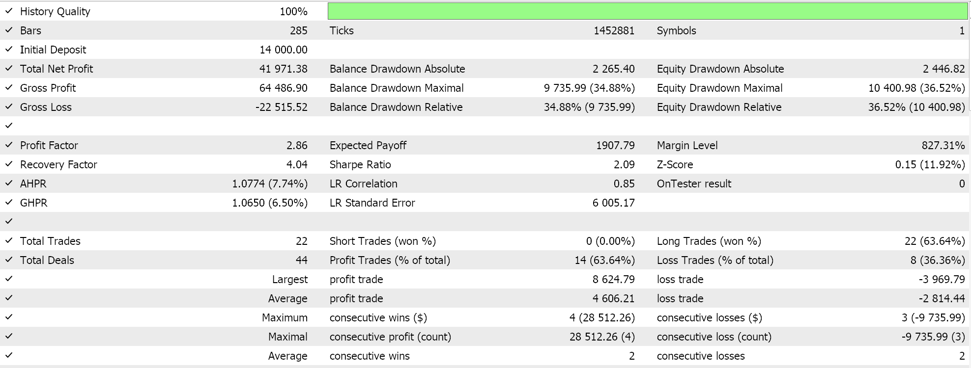
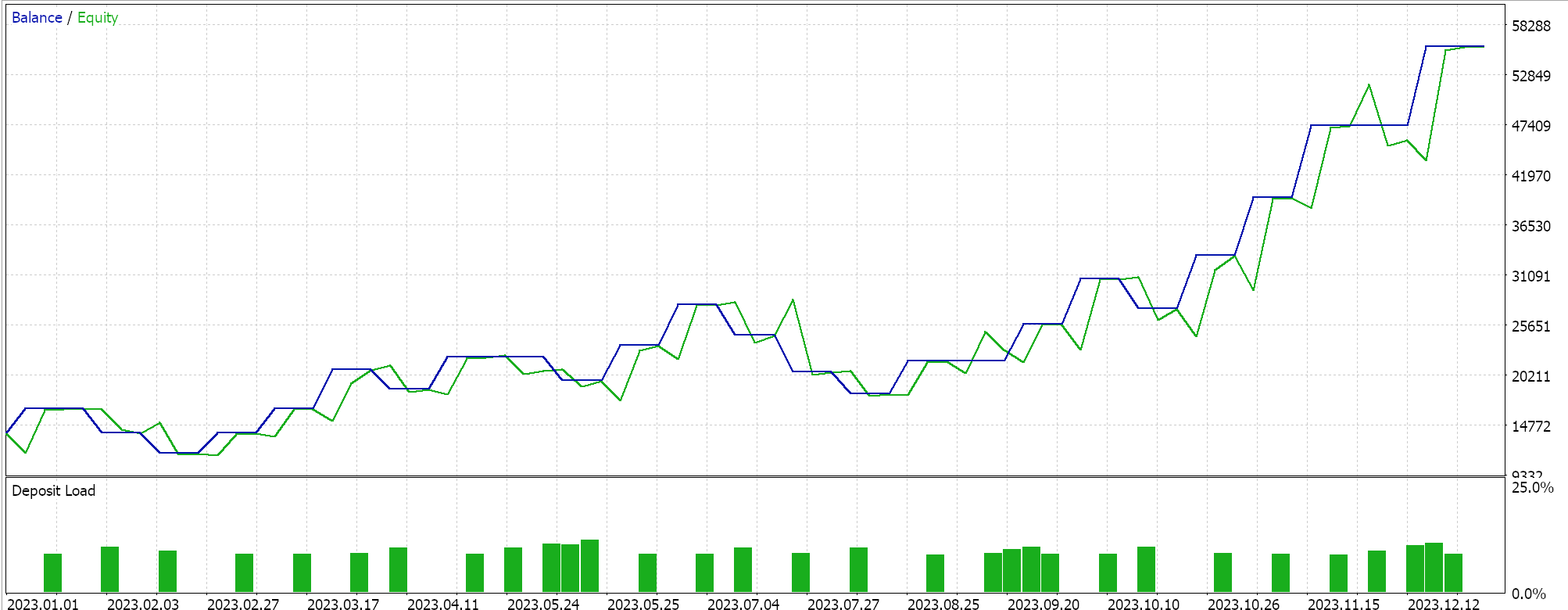
Other innovations of ADADELTA are reduction in hyperparameter sensitivity and the avoidance of diminishing learning rates. We do run tests with an ADADELTA learning rate on similar symbol, test period, and time frame as above and do get a variety of profitable results. Below is one of the reports:
One Cycle Learning Rate
This learning rate adjustment approach lacks the sophistication of the adaptive learning rate methods and is more akin to the cosine annealing format we considered in the last article. However, it is a bit simpler than the cosine annealing in that the learning rate gets increased and then reduced towards the end of the training session. This is implemented as follows:
      else if(m_learning_type == LEARNING_ONE_CYCLE)
      {  double _cycle_position = (double)((m_epochs - i) % (2 * m_epochs)) / (2.0 * m_epochs);
         if (_cycle_position <= 0.5)
         {  _learning_rate = m_min_learning_rate + (2.0 * _cycle_position * (m_learning_rate - m_min_learning_rate));
         }
         else
         {  _learning_rate = m_learning_rate - (2.0 * (_cycle_position - 0.5) * (m_learning_rate - m_min_learning_rate));
         }
      }
So, unlike the relatively complex approaches we have examined for this article in adjusting the learning rate, for one cycle the learning rate is simply initially increased in what is referred to as a warm-up phase, then it gets to the peak learning rate after which it then gets reduced in the cooling down phase which is the latter part of the training process. With the exception of cosine annealing, most learning rate approaches are keen on starting with a large learning rate and then reducing this value as more data is processed.
One cycle learning rate does something a bit in reverse, in that it starts at the minimum learning rate. The minimum learning rate and maximum learning rate are predefined input parameters, and the path or rate of change to the learning rate is influenced by the number of epochs or length of the training session. As we have done with the adaptive learning rates, we perform test runs with the one cycle learning rate and one of our test reports is presented below:
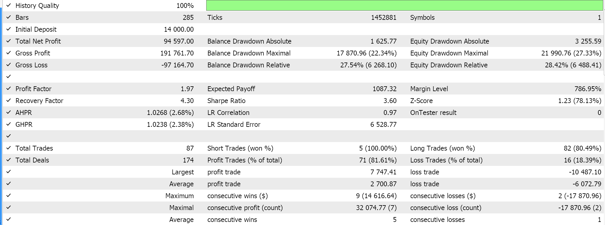
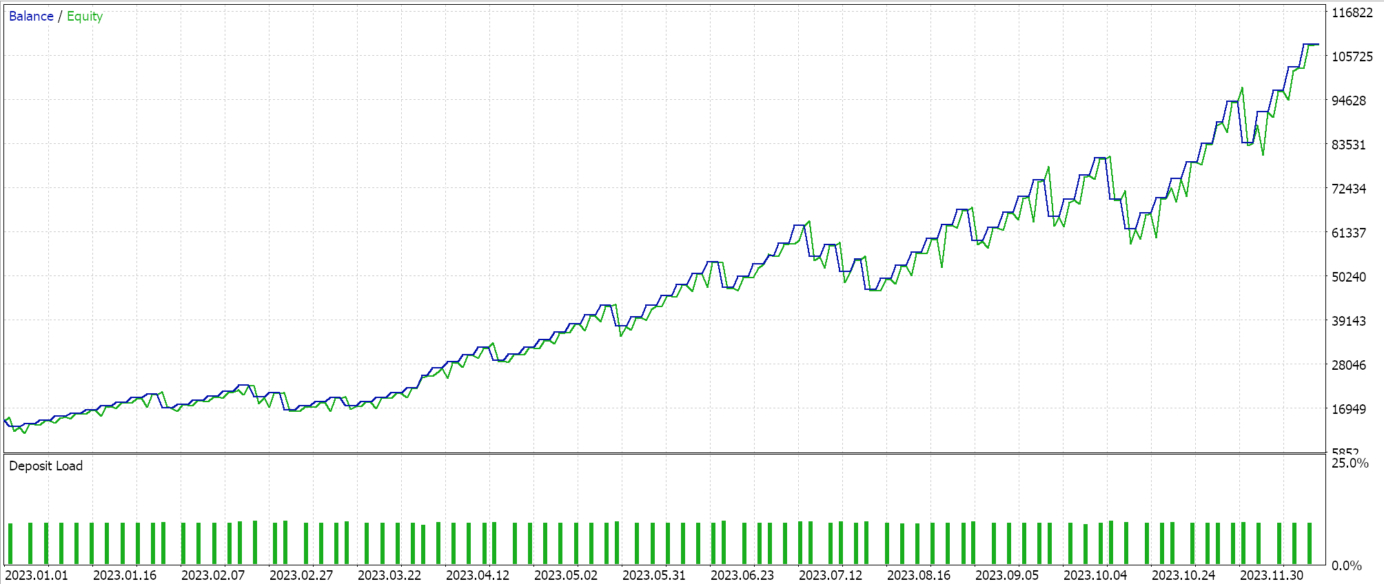
From our results above, despite a lack in proper batch normalization, by only tweaking the learning rate we are able to finally have some short trades opened. This is when forecasting raw symbol prices (given no batch normalization) and normalizing the long and short conditions in the same way we did when testing the adaptive learning rate methods. This once again demonstrates how sensitive the approach taken to using and adjusting the learning rate is to the performance of a neural network.
Conclusion
To sum up, learning rates are a crucial and very sensitive aspect of machine learning algorithms. We have examined the variations in implementing the various formats while focusing on the sequential innovations in each because most of the learning rate approaches were developed to improve earlier methods and approaches. This journey on improving these learning rates certainly is still in motion and continuing, however simpler bare-bones approaches like the one cycle learning rate should not be neglected as well as they can be quite impactful, as we’ve seen from some of our test results.
 Twitter Sentiment Analysis with Sockets
 Building A Candlestick Trend Constraint Model (Part 7): Refining our model for EA development
 Causal analysis of time series using transfer entropy
 Developing a Replay System (Part 42): Chart Trade Project (I)
- Free trading apps
- Over 8,000 signals for copying
- Economic news for exploring financial markets
You agree to website policy and terms of use
Dear Stephen,
Thank you for sharing your knowledge and work regarding this trading system!
I followed your article with great interest. However as I downloaded your attached zip file, it only consisted of:
1. Cmlp_ad.mqh
2. SignalWZ_29.mqh
3. mlp_learn_r.mq5
and within mlp_learn_r.mq5, it requires the following files:
1. Expert.mqh
2. TrailingNone.mqh
3. MoneyFixedMargin.mqh
may I know how we can obtain them please?
Without them... the EA does not work.
Thank you! I am very grateful!
they already exists under MQL include folder and you should add a header