MQL5 Wizard Techniques you should know (Part 30): Spotlight on Batch-Normalization in Machine Learning

Introduction

Batch normalization, a form of standardizing data before it is fed to neural network layers, is improving performance in the networks, and yet there is some disagreement as to why this is. While in the original paper on the subject, the reason stated was an internal covariate shift which can be understood as the mitigation of the effects of imbalances in input data of ‘upstream layers’ from having cascading effects on downstream layers, this more recent study claims improvements in empirical performance are down to smoothing since the intra-layer gradients have less variability given the normalization.

From a trader’s vantage, interest on WHY batch normalization makes a difference to a neural network’s performance is a reason plenty to develop and test systems that use it, and so that is our task at hand. There are three major forms of batch normalization that we’ll examine, namely Standard-Scaling, Feature-Scaling, and Robust-Scaling. Each of these is a very simple algorithm, we’ll run tests with Expert Advisors using each, and as a control we’ll also run tests with Expert Advisors that do not use batch normalization. So, our article will revert to the format we had been using before the last two articles (on learning rates) where we will now have descriptions of all three normalizations, then test reports on the same with a control, and finally a conclusion.

This article, like all in this series, highlights the use of wizard assembled Expert Advisors in testing out new ideas. Introductions on how this is done can be got from here and here for new readers, with those 2 articles providing some guidance on how to use the code attached at the end of this article. For this piece, we are using quite a few custom enumerations of data as optimizable inputs. The MQL5 inbuilt enumerations can be declared in the custom signal file’s header, and they will be automatically indicated as inputs and initialized as part of the signal filter. When the enumerations are custom though, placing them in the header will prevent the file from being visible (or recognizable) in the MQL5 wizard, meaning you cannot do the wizard assembly. The work around this we have, for now, is omitting them from the custom signal class header but having the parameters and their assignment functions declared within the signal class, as is always the case with any input parameter. Once the wizard assembly is completed, we then make manual changes to the roster of input parameters and also the initialization of the signal class to add this custom enumeration parameters.

There was a hack I had found around this that I think involved declaring the enumerations in the signal class itself, but I do not recall the specifics, so we will have to settle with this manual editing. Our test Expert Advisor has custom enumerations for learning rate type, adaptive learning rate type and most significantly for this article an enumeration on normalization types. The code of the latter is shared below:

enum Enormalize
{  NORMALIZE_NONE = -1,
   NORMALIZE_ROBUST = 0,
   NORMALIZE_FEATURE = 1,
   NORMALIZE_STANDARD = 2,
};

To use and optimize this enumeration within the Expert Advisor, we would need to manually add the enumeration parameters as inputs, as follows:

....

input ENUM_ACTIVATION_FUNCTION Signal_CMLP_ActivationType = AF_SIGMOID;  // CMLP(30,6,0.05,10,0.1,2,...) Activation Type
input Enormalize Signal_CMLP_NormalizeType   = NORMALIZE_FEATURE; // CMLP(30,6,0.05,10,0.1,2,...) Batch Normalisation Type
input Elearning Signal_CMLP_LearningType   = LEARNING_ADAPTIVE; // CMLP(30,6,0.05,10,0.1,2,...) Learning Type
input Eadaptive Signal_CMLP_AdaptiveType   = ADAPTIVE_GRADIENT; // CMLP(30,6,0.05,10,0.1,2,...) Adaptive Type

...

In addition, we would need to add the declared parameters to the instance of the custom signal, which is initialized as ‘filter0’. This is done as follows:

...

   filter0.ActivationType(Signal_CMLP_ActivationType);
   filter0.NormalizeType(Signal_CMLP_NormalizeType);
   filter0.LearningType(Signal_CMLP_LearningType);
   filter0.AdaptiveType(Signal_CMLP_AdaptiveType);

...

Once this is done, the wizard assembled Expert can be used normally with our custom signal class. Having introduced the 3 formats of normalization we are going to consider via the custom enumeration above, let's now have a brief overview of the subject, before taking a deeper look at each of the batch enumeration types, after which we’ll consider overall implementation in the custom signal class.

Arguments for Batch Normalization in Neural Networks

Officially, most of the benefits of batch normalization still evolve around the arguments made in the paper that brought it to light in 2015. Since there is now a debate on how it is able to achieve its empirical results, these original arguments may not necessarily carry the same weight as they did at inception. Nonetheless, we do present them here as an intro to the subject, at least. Batch normalization is touted to stabilize the training process by reducing the afore mentioned internal covariate shift. It improves convergence speed since the activations at each layer are ‘more standard’. In addition, it reduces sensitivity to the initialization weights used in a network before training. Initial weights tend to hold a disproportionate sway not only on the final weights that are arrived at, but also on how long the training process takes.

Furthermore, batch normalization acts as a regularizer by making the network less sensitive to the weights of some neurons. It also allows for the training of deep neural networks by reducing vanishing gradient problems. It decouples layer dependencies, it makes the training process invariant to changes in scale of input features, it enhances model generalization, it facilitates training different batch sizes, and is well-poised to experiment with various learning rate schedules. These are some of the touted advantages of batch normalization. Let’s now consider each type.

Feature Scaling

This form of normalization turns all the data in a vector at a layer into the range 0.0 to +1.0. The formula for this for each value in the vector is:

Where

• x’ is the normalized value
• x is the original de-normalized value
• min(x) is a function that returns the vector minimum
• max(x) returns the vector maximum

The implementation of this very simple algorithm would be straight forward in MQL5 as follows:

//+------------------------------------------------------------------+
//| Function to apply Feature-Scaling
//+------------------------------------------------------------------+
void Cnormalize::FeatureScaling(vector &Data)
{  vector _copy;
   _copy.Copy(Data);
   if(_copy.Max() - _copy.Min() > 0.0)
   {  for (int i = 0; i < int(Data.Size()); i++)
      {  Data[i] = (_copy[i] - _copy.Min()) / (_copy.Max() - _copy.Min());
      }
   }
}

Whenever selecting a normalization algorithm, the type of activation to be used at each layer is an important consideration. This is because not all activation functions output their results in the same range. Here is a tabulation of the various activation functions, available as an enumeration in MQL5, and their respective outputs ranges:

Activation Function	Output Range
Exponential Linear Unit (ELU)		(-1, ∞)
Exponential (Exp)		(0, ∞)
Gaussian Error Linear Unit (GELU)		(-∞, ∞)
Hard Sigmoid		[0, 1]
Linear		(-∞, ∞)
Leaky Rectified Linear Unit (Leaky ReLU)		(-∞, ∞)
Rectified Linear Unit (ReLU)		[0, ∞)
Scaled Exponential Linear Unit (SELU)		(-∞, ∞)
Sigmoid		(0, 1)
Softmax		(0, 1), sums to 1
Softplus		(0, ∞)
Softsign		(-1, 1)
Swish		(-∞, ∞)
Hyperbolic Tangent (Tanh)		(-1, 1)
Thresholded Rectified Linear Unit (Thresholded ReLU)		{0} ∪ [θ, ∞), where θ > 0

As is apparent, we have only 3 activation functions that provide outputs within a range similar to the batch normalization algorithm of feature scaling. These are Hard-Sigmoid, Sigmoid, and Soft max. Everything else is out of bounds. This matching of output ranges is vital if networks are to avoid the vanishing/ exploding gradient problems that occur a lot during training.

Hard sigmoid activation is a simple approximation of the sigmoid function that is defined by the following equation:

So, regardless of what input we have for x, the output will be range bound from 0.0 to +1.0. This matching to feature scaling ensures consistent and interpretable activations. In addition, the hard sigmoid is computationally efficient and therefore suitable for large and very deep networks like transformers.

The sigmoid activation function is arguably the most popular of all activations because of the way it minimizes problems of exploding gradients through the range-controlled output that still manages to maintain some degree of variability, unlike say the hard-sigmoid activation above. Its equation is as:

Where

• e is Euler’s constant
• x is the normalized value

The smoothness in its mapping aligns well with the normalized feature scale range. In addition, it does avoid issues with gradient saturation, since output values of 0.0 or 1.0 are rare.

Soft max activation, normalizes a class (or say a vector of data) such that all its values are not only in the 0.0 to 1.0 range, but in addition these normalized values when summed up add to 1.0. The equation that derives this is indicated below:

Where

• z i is the ith element of the input vector Z
• K is Z’s vector size
• e is Euler’s constant

Soft max is typically used in multi-class classification or the comparing of data points that have more than one dimension. The output does imply a probability distribution where no single output disproportionately dominates the others, creating a kind of even playing field. In addition, the summation to one ensures no large numbers are present which can create downstream computation problems in very deep networks or transformers.

So, hard-sigmoid, sigmoid and soft-max are the three suitable activation function algorithms for feature-scaling normalization since outputs of all three tend to match with the outputs of this batch normalization. Implementation of these algorithms in MQL5 is really straight forward, since all activation algorithms and their respective derivatives can be accessed from the inbuilt functions of the vector data type. Examples of this, are in the ‘Forward()’ and ‘Backward()’ functions that form part of the ‘Cmlp’ class that is attached to this article. Alternatively, official guidance is also available for both activation and derivative functions.

The implementation of feature scaling algorithm has already been highlighted above. It is a straight forward function that checks for zero divides by ensuring the maximum and minimum values in the vector are not the same. The scaling functions are very simple and this is important for minimizing compute given that a lot of networks can be very deep and in transformer format.

Robust Scaling

This form of normalization provides a bit more leeway in its output by giving values that slightly extend beyond -1.0 and +1.0 in certain conditions, but with most cases all data is often between -1.0 and +1.0. Exceptions to this are common, and they happen in instances where outliers are present such that their distance from the median is so large it exceeds the interquartile range. The governing equation for this, is as follows:

Where:

• x is the original value
• median(x) is the vector or class median
• IQR(x) is the 75^thpercentile minus the 25^thpercentile of the class.

While robust-scaling is less sensitive to outliers than feature scaling, it does not ignore them. In fact, outliers that fall far from the median are the ones that tend to provide normalized values whose magnitude is in excess of one. Also, in general if there is high variability in the data (the maximum to minimum range) when compared to the interquartile range; in other words, a situation where the data is predominantly centred around the median but with a gradually decreasing number towards the extremes such that the extreme values are not necessarily outliers. In these instances, also, the values closer to the extreme will have normalizations with magnitudes more than one.

From our table above on activation output ranges, it is clear that the ideal choice of activation functions to pair with robust scaling would be soft-sign activation or TANH activation. This is because their outputs, though a bit restrictive to the -1.0 to +1.0 range given the possible robust scaling outlier effects we have mentioned above, they are the best match from all the other activations. More importantly than that, though, is that these activation outputs do not produce any infinite values, so the risk of vanishing and exploding gradients is hugely mitigated.

Soft sign is defined by a very simple equation:

Where

• x is the data point in the class or vector
• |x| is the magnitude of this data

From its formula its clear x, or the data within a normalized vector, should ideally be floating point type and probably ranging in magnitude from 0.0 to 2.0. As x values scale up from 2.0 then the variability and therefore interpretation of the normalized data would be hampered. This points to the saturation of normalized values away from zero, but a smooth transitioning around the zero value. The symmetry and centring of values around zero aligns well with robust scaling. In addition, it has been observed that gradients from soft sign do not vanish as easily as those from other activation functions, such as the popular sigmoid activation. This can be very beneficial when performing extensive training on large data sets.

TANH activation is another -1.0 to +1.0 range bound algorithm that should work well, robust scaling. Its equation is given below:

Where

• x is a data point within the class or vector
• e is Euler’s constant

The TANH algorithm in form is very similar to sigmoid, with the obvious distinction being that it is centred around 0.0 while sigmoid is centred around 0.5. It also reportedly provides a smoother gradient than the sigmoid function. The sign range, as with soft-sign, makes it another ideal candidate to work with robust scaling, as we’ve seen above. Noisy data or datasets with a lot of outliers, which from a trader’s perspective could include price buffers of very volatile securities, are all ideal data sets to use with robust scaling and TANH activation. This stems from its ability to handle data sets with varied scales.

Implementation in MQL5 is as seamless as we say with the 3 activation functions for feature scaling above. The vector data type has both in built activation and derivative functions that output results to any vector that also serves as an input. This is outlined here and here respectively as already shared above.

The robust scaling algorithm is implemented in a normalize class in MQL5 as follows:

//+------------------------------------------------------------------+
//| Function to apply Robust-Scaling
//+------------------------------------------------------------------+
void Cnormalize::RobustScaling(vector &Data)
{  vector _copy;
   _copy.Copy(Data);
   if(_copy.Percentile(75) - _copy.Percentile(25) > 0.0)
   {  for (int i = 0; i < int(Data.Size()); i++)
      {  Data[i] = (_copy[i] - _copy.Median()) / (_copy.Percentile(75) - _copy.Percentile(25));
      }
   }
}

Like the feature scaling algorithm above, a check for zero divides is performed on the interquartile range. This once again is a simple algorithm for the efficiency reasons already highlighted above.

Standard Score

The standard score which is probably more common as the Z-Score is arguably the most popular normalization algorithm. In Wikipedia’s batch normalization page, it is the only used normalization function. It involves transforming a class or vector of data to values whose mean is 0 and whose standard deviation is 1. This is clearly different from the cases of feature scaling and robust scaling that we’ve considered above, where the output data’s range was in focus. Its equation is as follows:

Where

• Z is the normalized value
• μ is the mean
• σ is the standard deviation

From this equation we can therefore see that the output has an unbound range such that possible outputs can span from minus infinity to plus infinity. This ought to be a red flag, as exploding gradients can quickly become a problem, especially if the activation functions that are used with this also have unbound outputs. However, it does centre its outputs about zero, and this is good for stabilizing the training process for networks that used gradient descent. Furthermore, it is very effective when dealing with normally distributed data, as it ensures input data points contribute evenly to the learning process.

It does have cons as well though prime of which is sensitivity to outliers, presumption of a Gaussian distribution of the data, and as already stated an unbound output. The implementation of this standard score in MQL5 can be achieved as follows:

//+------------------------------------------------------------------+
//| Function to apply Standard-Score
//+------------------------------------------------------------------+
void Cnormalize::StandardScore(vector &Data)
{  vector _copy;
   _copy.Copy(Data);
   if(_copy.Std() != 0.0)
   {  for (int i = 0; i < int(Data.Size()); i++)
      {  Data[i] = (_copy[i] - _copy.Mean()) / _copy.Std();
      }
   }
}

Interestingly, this is not yet a standard feature amongst the MQL5 functions. In avoiding zero divides for all these three normalization functions, rather than checking for a zero denominator, it is also common to add a small non-zero double value at the bottom that is often referred to as epsilon. This practice though when done with feature scaling or robust scaling can lead to very large normalized values in the event the would-be denominator was zero.

Normalization Transformer

Once layer input data has been normalized by either feature-scaling, or robust-scaling, or the standard score, the outputs from these normalization gets fed into the batch normalization transformer. It’s also a relatively straight forward function that is defined by the following equation:

Where

• y represents the output in the vector at index i
• x is the previously normalized data point at index i
• Gamma and Beta are optimizable floating-point parameters

Coding this also does not take too much as we can have this in MQL5 as follows:

//+------------------------------------------------------------------+
//| Batch Normalizing Transform
//+------------------------------------------------------------------+
void Cnormalize::Transform(Enormalize Type, vector &Output, vector &BatchTransform, vector &Beta, vector &Gamma)
{  if(Type != NORMALIZE_NONE)
   {  if(Type == NORMALIZE_STANDARD)
      {  StandardScore(Output);
      }
      else if(Type == NORMALIZE_FEATURE)
      {  FeatureScaling(Output);
      }
      else if(Type == NORMALIZE_ROBUST)
      {  RobustScaling(Output);
      }
      //Transformer
      BatchTransform.Init(Output.Size());
      BatchTransform.Fill(0.0);
      for(int i = 0; i < int(Output.Size()); i++)
      {  BatchTransform[i] = (Gamma[i] * Output[i]) + Beta[i];
      }
   }
}

Arguments for taking the normalization output through this transformer are mainly five. Firstly, it restores the representative power of the original non-normalized data by introducing flexibility and recalibration. Flexibility because after transformation the output data may not necessarily be in an optimal state to facilitate the network’s learning. For instance, when using standard score normalization, the output data of each vector always has a mean of 0 and standard deviation of 1. This and other similar cases may be too extreme for the network to train effectively. That’s why the introduction of learnable/ optimizable parameters beta and gamma can help re-calibrate this data sets to an optimal form for training.

Secondly, in cases where the initial normalization function has potentially unbound outputs, like, again, the standard score, this normalization transformer can help avert vanishing and exploding gradients. This would be achieved by fine-tuning beta and gamma. Thirdly, it is argued that the transformer maintains variance for effective learning through variance scaling. The gamma parameter can adjust the variance of the normalized outputs since it is a direct multiple. With this ability to adjust this variance, the learning process can be fine-tuned to suit the architecture of the network.

In addition, the transformer can enhance the learning dynamics of a network by having the network adapt to the data that often leads to improvements in convergence. The optimizable beta and gamma parameters once again guide this process such that the data is scaled to better use the network layer number and size settings, with the end result of this being fewer training epochs required to achieve ideal results. Finally, a regularization from scaling and shifting the outputs of the normalized data is argued to work like drop out regularization. Regularization is meant to nudge the network to learn more of the underlying patterns in a dataset and less of the noise so the beta and gamma parameters, which are vector parameters, are unique to each layer. This customization on a parameter basis does in addition to regularizing the network, also the covariate shift which we talked about in the introduction can be realized better thanks to the parameter specific action of beta and gamma.

Strategy Test Results

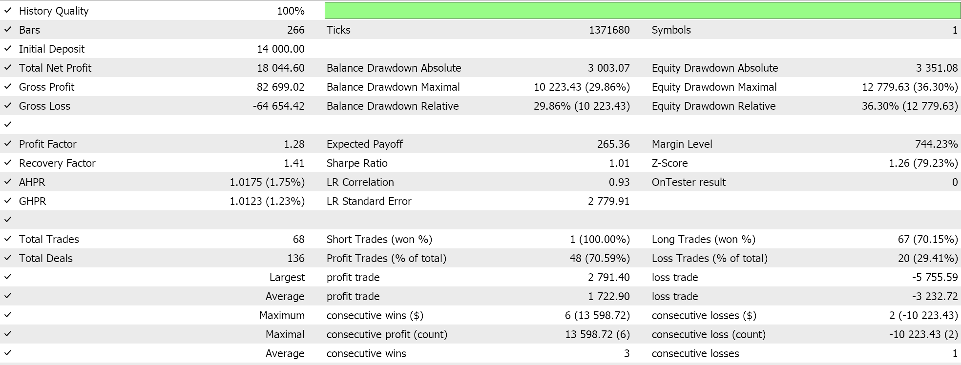
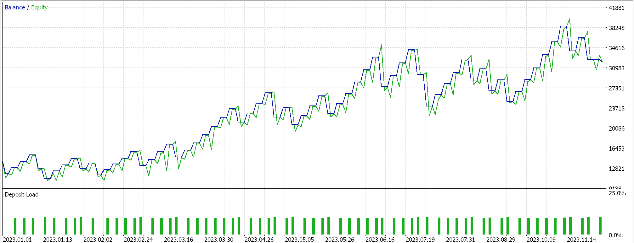
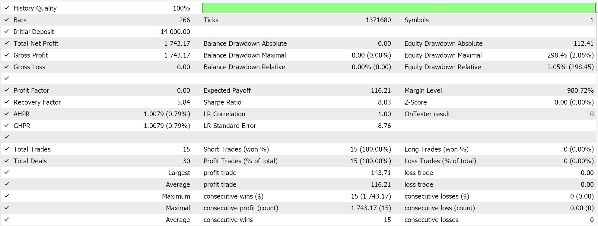
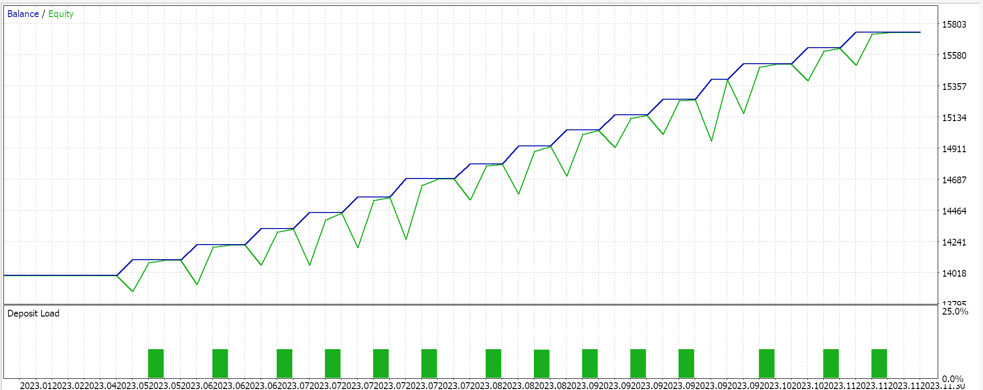
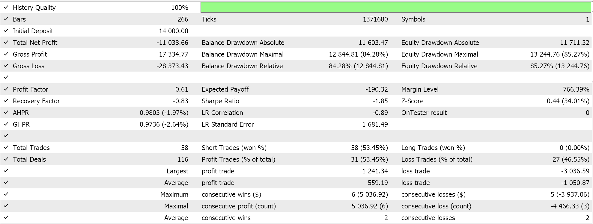
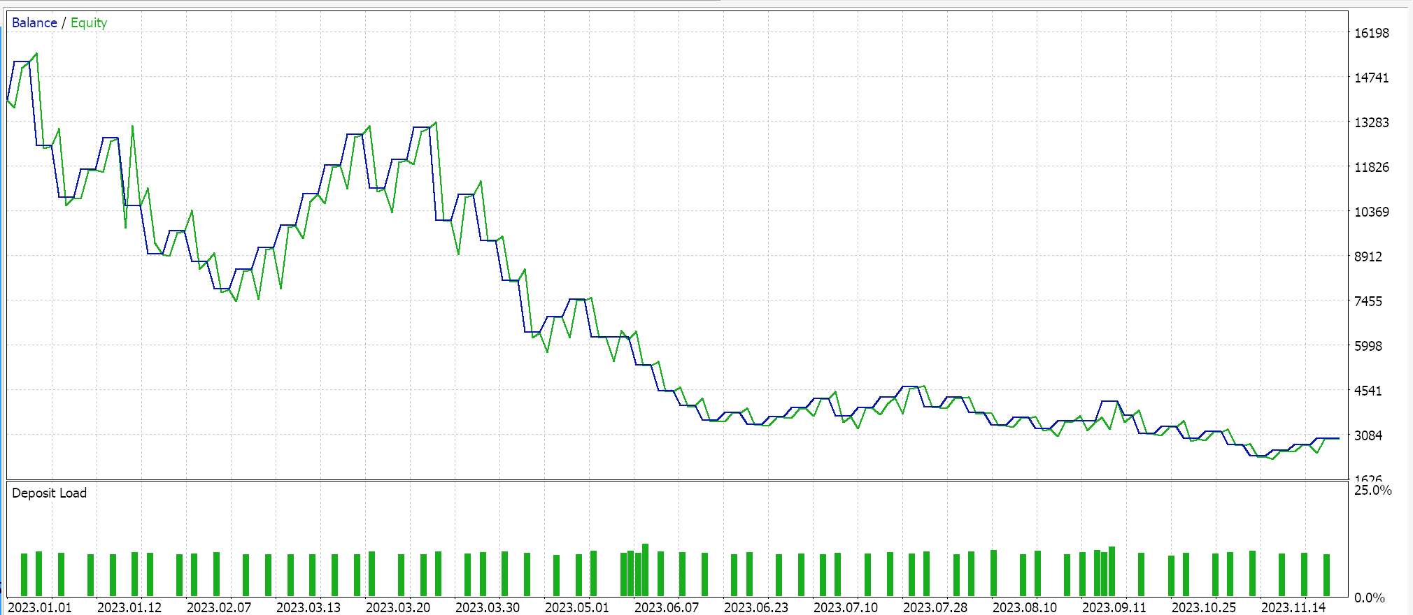
For testing, we are using the symbol EURJPY on the daily time frame for the year 2023. The standard score normalization, being with unbound data, does not necessarily have a suitor activation function. One can use the bound activation functions we have mentioned in this article, however that testing is left to the reader. For our purposes, we are testing only the robust scaling normalization and feature scaling normalization. We paired these with soft-sign and sigmoid activation, respectively.

For feature scaling, we had the following results:

For robust scaling, we had:

As a control, we perform tests with the Expert Advisor running identical settings but without normalization. Below are our results:

Conclusion

So, to sum up our key findings, batch normalization is parameter intense and therefore compute expensive. Extra care needs to be taken when selecting normalization algorithms to use and although standard score is very popular and common, it has unbound outputs which can lead to very large gradients which hamper convergence and slow down the entire training process. If, however, alternative normalization algorithms that have bound outputs like feature scaling or robust scaling are used and these are paired with their respective activation functions that have similar bound outputs, then the training process can be accelerated. Speed unfortunately is a key consideration here because as already mentioned batch normalization involves a lot of parameters and is compute-intense, therefore extra care needs to be made in pairing normalization algorithms to activation functions plus having optimal network layers and sizes.