Integrating MQL5 with data processing packages (Part 2): Machine Learning and Predictive Analytics

Introduction

In this article we focus specifically on Machine Learning (ML) and Predictive Analytics. Data processing packages opens new frontiers for quantitative traders and financial analysts. By embedding machine learning capabilities within MQL5, traders can elevate their trading strategies from traditional rule-based systems to sophisticated, data-driven models that continuously adapt to evolving market conditions.

The process involves using Python’s powerful data processing and machine learning libraries like scikit-learn in conjunction with MQL5. This integration allows traders to train predictive models using historical data, test their effectiveness using back-testing techniques, and then deploy those models to make real-time trading decisions. The flexibility to blend these tools enables the creation of strategies that go beyond typical technical indicators, incorporating predictive analytics and pattern recognition that can significantly enhance trading outcomes.

Gather Historical Data

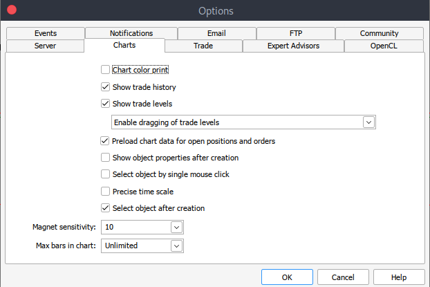
To get started we need historical data from MetaTrader 5 saved in .csv format, so simply launch your MetaTrader platform and at the top of your MetaTrader 5 pane/panel navigate to > Tools and then > Options and you will land to the Charts options. You will then have to select the amount of Bars in the chart you want to download. It's best to choose the option of unlimited bars since we'll be working with date and we wouldn't know how many bars are there in a given period of time.

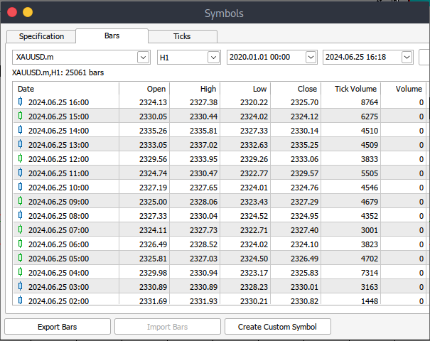
After that you will now have to download the actual data. To do that you will have to navigate to > View and then to  > Symbols and you will land on the Specifications tab simply navigate to > Bars or Ticks depending on what kind of data want to download. Proceed and enter the start and end date period of the historical data you want to download, after that click on the request button to download the data and save it in the .csv format.

After all those steps you would have successfully download historical data from your MetaTrader trading platform. Now you need to download and set up the Jupyter Lab environment for analysis. To download and set up Jupyter Lab you can head to their official website and follow simple step to download it. Depending on the type of operating system you use, you will have variety of options of whether to install using pip, conda or brew.

Process MetaTrader 5 Historical Data on Jupyter Lab

To successfully load your MetaTrader 5 historical data on Jupyter Lab you will have to know the folder that you had selected to download the data to, and then on Jupyter Lab simply navigate to that folder.To get started you will have to load the data and inspect the column names. We have to inspect the column names so that we handle the columns correctly and avoid errors that might arise if we use the wrong column name.

python code:

import pandas as pd

# assign variable to the historical data
file_path = '/home/int_junkie/Documents/ML/predi/XAUUSD.m_H1_201510010000_202408052300.csv'

data = pd.read_csv(file_path, delimiter='\t')

# Display the first few rows and column names
print(data.head())
print(data.columns)

Output:

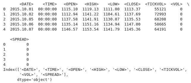
We are working with MetaTrader 5 historical data from the year 2015 to 2024, that's about 9 years of historical data. This kind of data helps to capture broad market cycles. The data set is likely to capture different market phases, which will enable better understanding and modeling of these cycles. Longer datasets reduce likelihood of over fitting by providing a more comprehensive range of scenarios.

A model trained on a broader dataset is more likely to generalize well to unseen data, especially if the dataset is that of lower time frame like 1H. This is particularly important in time series analysis, where having more observations enhances the reliability of the results. For instance, you can detect secular trends (long-term market directions) or recurring seasonal effects that are relevant for forecasting.

Line Plot From Historical Data

data.plot.line(y = "<CLOSE>", x = "<DATE>", use_index = True)

Output:

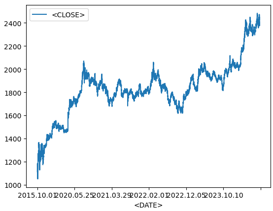
We use the code above when visualizing time-series data, such as financial asset over time. If your Data-Frame's index already contains dates, you can skip specifying 'x="<DATE>"' and just use 'use_index=True'.

del data["<VOL>"]
del data["<SPREAD>"]

We then delete the specified columns from our historical data, we use the pandas library to delete these columns.

data.head()

Output:

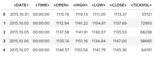
From the output above we can see that indeed the specified columns were deleted.

# We add a colunm for tommorows price
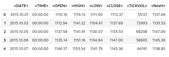
data["<NexH>"] = data["<CLOSE>"].shift(-1)

1. 'data["<NexH>"]':

• This adds a new column called '"<NexH>"' (NEXT HOUR) to the 'data' Data-Frame. The value in this column will represent the closing prices for the next hour relative to each row.

2. 'data["<CLOSE>"].shift(-1)':

• 'data["<CLOSE>"]' refers to the existing column in the Data-Frame that contains the closing prices of for each date-time.
• The '.shift(-1)' method shifts the date-time in the "<CLOSE>" column up by 1 row (because the argument is '-1'), which effectively moves each value to the previous row.
• As a result, the value that originally corresponded to a particular date will now appear in the row corresponding to the previous date.

Output:

data["<TRGT>"] = (data["<NexH>"] > data["<CLOSE>"]).astype(int)

data

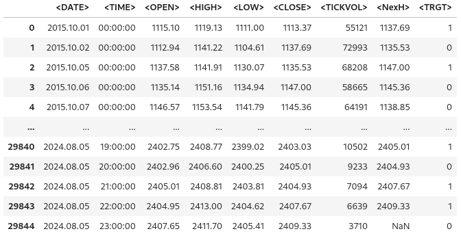
We use then use the code above to create new column in the 'data' Data-Frame that contains binary values (0 or 1) indicating whether the next period's high price ('"NexH"') is greater than the current closing price ('"<CLOSE>"').

1. 'data["<TRGT>"]':

• This is the new column called '"<TRGT>"' (TARGET) in the 'data' Data-Frame. This column will store the binary target values (0 or 1) based on a condition.

2. '(data["<NexH>"] > data["<CLOSE>"])':

• This expression compares the value in the '"<NexH>"' column (next period's high price) to the value in the '"<CLOSE>"' column (current closing price) for each row.
• This is a boolean series, where each value is either 'True' (if the next high is greater than the current close) or 'False' (of not).

3. '.astype(int)':

• This function converts the boolean values ('True' or 'False') into integers ('1' or '0', respectively).
• 'True' becomes '1', and 'False' becomes '0'.

Output:

from sklearn.ensemble import RandomForestClassifier

model = RandomForestClassifier(n_estimators = 50, min_samples_split = 50, random_state = 1)

train = data.iloc[:-50]
test = data.iloc[-50:]

predictors = ["<CLOSE>","<TICKVOL>", "<OPEN>", "<HIGH>", "<LOW>"]
model.fit(train[predictors], train["<TRGT>"])

Output:

1. Importing the Random Forest Classifier:

• The 'Random-Forest-Classifier' is an assemble machine learning model that builds multiple decision trees and merges their outputs to improve predictive accuracy and control over-fitting.

2. Model Initialization:

• 'estimator' specifies the number of decision trees in the forest. In this case, the model will build 50 trees.
• 'min-sample-split' sets the minimum of samples required to split an internal node. A higher value reduces over-fitting by ensuring that splits only occur when enough data is available.
• 'random-state' fixes the random seed to unsure reproducibility of results. Using the same seed (e.g, '1') will yield the same results each time the code is run.

3. Splitting the Data into Training and Test Sets:

• 'data.iloc[:-50]' selects all rows except the last 50 as the training data.
• 'data.iloc[-50:]' selects the last 50 rows as the test data
• This split is commonly used in time-series data, where the model is trained on historical data and tested on the most recent data evaluate performance on future predictions.

4. Specifying the Predictor Variables:

• The 'predictors' list contains the column names representing the features used by the model to make predictions. These include (''"<CLOSE>", '"<TICKVOL>"', '"<OPEN>"', '"<HIGH>"', and '"<LOW>"').
  

The code prepares a Random Forest classifier to predict future market behavior based on past data. The model is trained using features like closing price, tick volume, and others. After splitting the data into training and test set, the model is fitted to the training data, learning from the historical patterns to make future predictions.

Measure the accuracy of the model

from sklearn.metrics import precision_score

prcsn = model.predict(test[predictors])

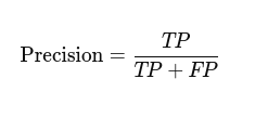
We import the function 'precision-score' from the 'sklearn.metrics' module. The precision score is a metric used to evaluate classification models, particularly useful when the classes are imbalanced. It measures how many of the predicted positive results are actually positive. High precision indicates low positive rates.

prcsn = pd.Series(prcsn, index = test.index)

We then convert the predictions ('prcsn') into a Pandas 'Series' while preserving the index from the test dataset.

precision_score(test["<TRGT>"], prcsn)

We get the precision of the model's predictions by comparing the actual target values in the test set with the predicted values.

Output:

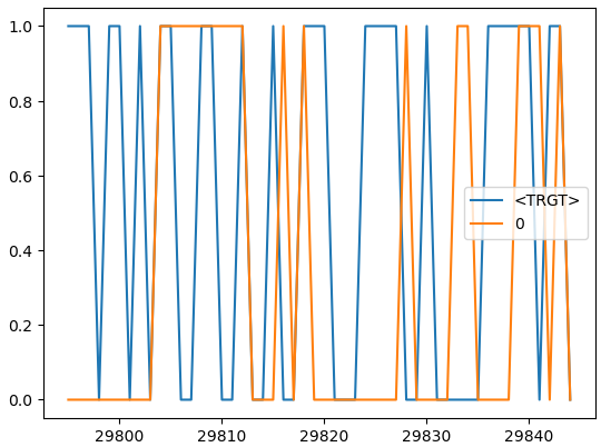
cmbnd = pd.concat([test["<TRGT>"], prcsn], axis = 1)

cmbnd.plot()

We combine the actual target values and the model's predicted values into a single Data-Frame for easier analysis.

Output:

def predors(train, test, predictors, model):
    model.fit(train[predictors], train["<TRGT>"])
    prcsn = model.predict(test[predictors])
    prcsn = pd.Series(prcsn, index = test.index, name = "Predictions")
    cmbnd = pd.concat([test["<TRGT>"], prcsn], axis = 1)
    return cmbnd

This function takes in training and test dataset, a list of predictor variables, and a machine learning model. The function trains the model on the training data, makes predictions on the test data, and returns a Data-Frame that contains both the actual target values and the predicted values side-by-side.

def backtestor(data, model, predictors, start = 2500, step = 250):
    all_predictions = []

    for i in range(start, data.shape[0], step):
        train = data.iloc[0:i].copy()
        test = data.iloc[i:(i + step)].copy()
        predictions = predors(train, test, predictors, model)
        all_predictions.append(predictions)
    return pd.concat(all_predictions)

This function performs a rolling back-test on a time series dataset using a machine learning model. The back-test evaluates the model’s performance by simulating predictions as if they were made in a real-world trading environment, where data is gradually revealed over time.

predictions = backtestor(data, model, predictors)

Runs the 'backtestor' function using the specified dataset ('data'), machine learning model ('model'), and predictor variables ('predictors'). It performs a rolling back-test, and the resulting predictions are stored in the variable 'predicitions'.

predictions["Predictions"].value_counts()

We count the number of occurrences of each unique value in the '"Predictions"' column of the 'prediction' Data-Frame.

Output:

precision_score(predictions["<TRGT>"], predictions["Predictions"])

Calculates the precision of the model's prediction. Precision is a metric that measures the accuracy of positive predictions.

Output:

predictions["<TRGT>"].value_counts() / predictions.shape[0]

Calculates the proportion of each unique value in `"<TRGT>"` column relative to the total number of predictions.

Output:

horizons = [2, 5, 55, 125, 750]
new_predictors = []

# Ensure only numeric columns are used for rolling calculations
numeric_columns = data.select_dtypes(include=[float, int]).columns

for i in horizons:
    # Calculate rolling averages for numeric columns only
    rolling_averages = data[numeric_columns].rolling(i).mean()
    
    # Generate the ratio column
    ratio_column = f"Close_Ratio_{i}"
    data[ratio_column] = data["<CLOSE>"] / rolling_averages["<CLOSE>"]
    
    # Generate the trend column
    trend_column = f"Trend_{i}"
    data[trend_column] = data["<TRGT>"].shift(1).rolling(i).sum()
    
    new_predictors += [ratio_column, trend_column]
data

Generates new features based on rolling averages and trends over different time horizons. The additional predictors help improve models performance by providing it with more information about the market over varying periods.

Output:

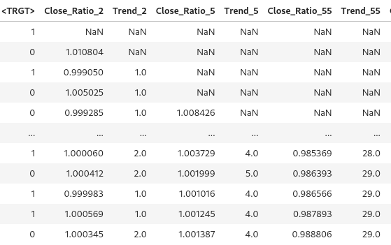
data = data.dropna()

We drop any row in the Data-Frame with missing values.

def predict(train, test, predictors, model):
    model.fit(train[predictors], train["<TRGT>"])
    prcsn = model.predict_proba(test[predictors])[:1]
    prcsn[prcsn >= .6] = 1
    prcsn[prcsn < .6] = 0
    prcsn = pd.Series(prcsn, index = test.index, name = "Predictions")
    cmbnd = pd.concat([test["<TRGT>"], prcsn], axis = 1)
    return cmbnd

The model is trained on the training dataset using the selected predictors and target variable. For threshold and predictions, we apply a custom threshold of 0.6. If the probability for class1 is 0.6 or higher, the model predicts "1". Otherwise if predicts "0". This adjustment allows the model to be more conservative, requiring higher confidence before signaling a trade.

predictions = backtestor(data, model, new_predictors)

predictions["Predictions"].value_counts()

precision_score(predictions["<TRGT>"], predictions["Predictions"])

Output:

Our precision score went up slightly, 0.52 if we round up.

Train the Model and export it to ONNX

import pandas as pd
from sklearn.ensemble import RandomForestClassifier
from sklearn.model_selection import train_test_split
import onnx
import skl2onnx
from skl2onnx import convert_sklearn
from skl2onnx.common.data_types import FloatTensorType

# Load and preprocess your data (example)
# Replace this with your actual data loading process
#data = pd.read_csv('your_data.csv')  # Replace with your actual data source
#data = data.dropna()

# Define predictors and target
predictors = ["<CLOSE>", "<TICKVOL>", "<OPEN>", "<HIGH>", "<LOW>"]
target = "<TRGT>"

# Split data into train and test sets
train, test = train_test_split(data, test_size=0.2, shuffle=False)

# Define and train the model
model = RandomForestClassifier(n_estimators=50, min_samples_split=50, random_state=1)
model.fit(train[predictors], train[target])

# Export the trained model to ONNX format
initial_type = [('float_input', FloatTensorType([None, len(predictors)]))]
onnx_model = convert_sklearn(model, initial_types=initial_type)

# Save the ONNX model to a file
with open("random_forest_model.onnx", "wb") as f:
    f.write(onnx_model.SerializeToString())

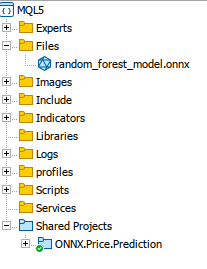
We train our model, and it is converted and exported and saved on ONNX format using `skl2onnx`. We the copy our saved model to MQL5 'Files' folder where we will be able to access it.

Putting it all together on MQL5

Load the model on the Oninit().

#include <Trade/Trade.mqh>
#define   ModelName          "RandomForestClassifier"
#define   ONNXFilename       "random_forest_model.onnx"

// Single ONNX model resource
#resource "\\Files\\random_forest_model.onnx" as const uchar ExtModelDouble[];

input double lotsize = 0.1;     // Trade lot size
input double stoploss = 20;     // Stop loss in points
input double takeprofit = 50;   // Take profit in points

// Trading functions
CTrade m_trade;

The includes  and global variables on the global scope. We also specify that the ONNX model is embedded to MQL5 as a binary resource. The `#resource` is used to include external files.

//+------------------------------------------------------------------+
//| Run classification using double values                           |
//+------------------------------------------------------------------+
bool RunModel(long model, vector &input_vector, vector &output_vector)
{
    ulong batch_size = input_vector.Size() / 5; // Assuming 5 input features
    if (batch_size == 0)
        return (false);

    output_vector.Resize((int)batch_size);

    // Prepare input tensor
    double input_data[];
    ArrayResize(input_data, input_vector.Size());

    for (int k = 0; k < input_vector.Size(); k++)
        input_data[k] = input_vector[k];

    // Set input shape
    ulong input_shape[] = {batch_size, 5}; // 5 input features for each prediction
    OnnxSetInputShape(model, 0, input_shape);

    // Prepare output tensor
    double output_data[];
    ArrayResize(output_data, (int)batch_size);

    // Set output shape (binary classification)
    ulong output_shape[] = {batch_size, 2}; // Output shape for probability (0 or 1)
    OnnxSetOutputShape(model, 0, output_shape);

    // Run the model
    bool res = OnnxRun(model, ONNX_DEBUG_LOGS, input_data, output_data);

    if (res)
    {
        // Copy output to vector (only keeping the class with highest probability)
        for (int k = 0; k < batch_size; k++)
            output_vector[k] = (output_data[2 * k] < output_data[2 * k + 1]) ? 1.0 : 0.0;
    }

    return (res);
}

This function `RunModel` an ONNX model the we have trained to perform binary classifications. The function determines the predicted class (0 or 1) based on which class has the higher probability and stores the results in an output vector.

//+------------------------------------------------------------------+
//| Generate input data for prediction                               |
//+------------------------------------------------------------------+
vector input_data()
{
    vector input_vector;
    MqlRates rates[];

    // Get the last 5 bars of data
    if (CopyRates(Symbol(), PERIOD_H1, 5, 1, rates) > 0)
    {
        input_vector.Resize(5 * 5); // 5 input features for each bar

        for (int i = 0; i < 5; i++)
        {
            input_vector[i * 5] = rates[i].open;
            input_vector[i * 5 + 1] = rates[i].high;
            input_vector[i * 5 + 2] = rates[i].low;
            input_vector[i * 5 + 3] = rates[i].close;
            input_vector[i * 5 + 4] = rates[i].tick_volume;
        }
    }

    return (input_vector);
}

//+------------------------------------------------------------------+
//| Check if there is a new bar                                      |
//+------------------------------------------------------------------+
bool NewBar()
{
    static datetime last_time = 0;
    datetime current_time = iTime(Symbol(), Period(), 0);

    if (current_time != last_time)
    {
        last_time = current_time;
        return (true);
    }
    return (false);
}

//+------------------------------------------------------------------+
//| Check if a position of a certain type exists                     |
//+------------------------------------------------------------------+
bool PosExists(int type)
{
    for (int i = PositionsTotal() - 1; i >= 0; i--)
    {
        if (PositionGetInteger(POSITION_TYPE) == type && PositionGetString(POSITION_SYMBOL) == Symbol())
            return (true);
    }
    return (false);
}

//+------------------------------------------------------------------+
//| Script program initialization                                    |
//+------------------------------------------------------------------+
int OnInit()
{
    Print("Initializing ONNX model...");

    // Initialize the ONNX model
    long model = OnnxCreateFromBuffer(ExtModelDouble, ONNX_DEFAULT);
    if (model == INVALID_HANDLE)
    {
        Print("Error loading ONNX model: ", GetLastError());
        return INIT_FAILED;
    }

    // Store the model handle for further use
    GlobalVariableSet("model_handle", model);
    return (INIT_SUCCEEDED);
}

//+------------------------------------------------------------------+
//| Expert tick function                                             |
//+------------------------------------------------------------------+
void OnTick()
{
    if (NewBar()) // Trade at the opening of a new candle
    {
        vector input_vector = input_data();
        vector output_vector;

        // Retrieve the model handle
        long model = GlobalVariableGet("model_handle");
        if (model == INVALID_HANDLE)
        {
            Print("Invalid model handle.");
            return;
        }

        bool prediction_success = RunModel(model, input_vector, output_vector);
        if (!prediction_success || output_vector.Size() == 0)
        {
            Print("Prediction failed.");
            return;
        }

        long signal = output_vector[0]; // The predicted class (0 or 1)

        MqlTick ticks;
        if (!SymbolInfoTick(Symbol(), ticks))
            return;

        if (signal == 1) // Bullish signal
        {
            if (!PosExists(POSITION_TYPE_BUY)) // No buy positions exist
            {
                if (!m_trade.Buy(lotsize, Symbol(), ticks.ask, ticks.bid - stoploss * Point(), ticks.ask + takeprofit * Point())) // Open a buy trade
                    Print("Failed to open a buy position, error = ", GetLastError());
            }
        }
        else if (signal == 0) // Bearish signal
        {
            if (!PosExists(POSITION_TYPE_SELL)) // No sell positions exist
            {
                if (!m_trade.Sell(lotsize, Symbol(), ticks.bid, ticks.ask + stoploss * Point(), ticks.bid - takeprofit * Point())) // Open a sell trade
                    Print("Failed to open a sell position, error = ", GetLastError());
            }
        }
    }
}

//+------------------------------------------------------------------+
//| Script program deinitialization                                  |
//+------------------------------------------------------------------+
void OnDeinit(const int reason)
{
    // Release the ONNX model
    long model = GlobalVariableGet("model_handle");
    if (model != INVALID_HANDLE)
    {
        OnnxRelease(model);
    }
}

During the initialization the model is loaded and its handle is stored for later use. In the 'OnTick()' function, the script runs the model when a new bar is detected. We use the model's prediction (0 for bearish and 1 for bullish), and execute trades accordingly. Buy trades are place when the model predicts a bullish trend, while sell trades are placed for a bearish trend.

Conclusion

In summary, we have used data processing package (Jupyter Lab) to process historical data, developed and trained the model using machine learnig to be able to make predictions. We have explored crucial steps that are necessary for a seamless integration and operation. We then focused on loading and handling the model within MQL5 by embedding it as a resource and ensuring that the model is properly initialized and available during runtime.

In conclusion, we have integrated an ONNX model into an MQL5 trading environment to enhance decision-making using machine learning. The process began with loading the model into the MQL5 environment. We then configured the Expert Advisor to gather relevant market data, preprocess it into feature vectors, and feed it into the model for predictions. Logic was designed to execute trades based on the model's output. Positions are only opened when a new bar is detected and no conflicting trades are active. Additionally, the system handles position checks, error management, and resource de-allocation to ensure a robust and efficient trading solution. This implementation demonstrates a seamless blend of financial analysis and AI-driven insights, enabling automated trading strategies that adapt to market conditions in real-time.

References

Create a model