MQL5 Wizard Techniques you should know (Part 26): Moving Averages and the Hurst Exponent

Introduction

We continue this series on techniques with the MQL5 wizard that focus on alternative methods in Financial time series analysis for the benefit of traders. For this article, we consider the Hurst Exponent. This is a metric which tells us whether a time series has a high positive autocorrelation or a negative autocorrelation over the long term. The applications of this measurement can be very extensive. How would we use it? Well, firstly, we’d calculate the Hurst exponent to determine if the market is trending (which would typically give us a value greater than 0.5) or if the market is mean-reverting/ whipsawed (that would give us a value less than 0.5). For this article, since we are in a ‘season of looking at moving averages’ given the last pair of articles, we will marry the Hurst Exponent information with the relative position of the current price to a moving average. The relative position of price to a moving average can be indicative of price’s next direction, with one major caveat.

You would need to know if the markets are trending, or they are ranging (mean-reverting). Since we can use the Hurst Exponent to answer this question, it follows we would simply look at where price is relative to the average and then place a trade. However, even this may still be a bit of a rush, given that ranging markets tend to be better studied on shorter time periods than trending markets that are more apparent when looking at much longer time periods. It is for this reason that we would need two separate moving averages to weigh the relative position of price before a definitive condition can be assessed. These will be a fast-moving average for ranging or mean-reverting markets, and a slow-moving average for trending markets, as determined by the Hurst Exponent. So, each market type as set by the Exponent would have its own moving average. This article therefore is going to look at Rescaled Range Analysis as a means at estimating the Hurst Exponent. We will go through the estimation process a step at a time and conclude with an Expert Signal Class that implements this Exponent.

Splitting Up the Time Series

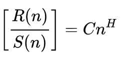
As per Wikipedia, the formula for the Hurst Exponent is presented as:

Where

• n is the size of the analysed sample
• R() is the re-scaled range of the sample
• S() is the standard deviation of the sample
• C is a constant
• H is the Hurst Exponent

This formula inherently presents us with 2 unknowns, and the work around this, to find both the constant C and our sought exponent H, is by regressing multiple segments of the sampled set. H is a power which from arithmetic means we take logarithms on both sides of the equation in order to solve for H, and this is our last step, as we shall see below. So, the very first step is to identify or define segments within the sampled data.

The minimum number of segments we can get from any sample is 2. The maximum we can get from a sample depends on the sample size, and the rudimentary formula is the sample size divided by 2. Now we are looking for two unknowns, meaning we need more than a pair of points so as to have the minimum 2 equations as is practice. The number of equations or pairs of points we can generate from a sample is given by half the sample size minus 1. So, a sample size of 4 data points will only generate one pair of points for regression, which will clearly not be enough to find the Hurst Exponent and the C constant.

A sample though, with 6 data points can generate the minimum 2 pairs of points that could be used to estimate the exponent and constant. In practice, we want the sample size to be as large as possible because as mentioned in the definition, the Hurst Exponent is a ‘long term’ property. Also, the Wikipedia formula shared above applies for samples as n tends towards infinity. So, it’s important that the sample size is as large as possible in order to estimate a more representative Hurst Exponent.

The splitting of the sample into segments where each split/ segment set generates a single pair of points is the very ‘first step’. I use ‘first step’ because in the approach we use for this article, as is shown in the source code below, we do don’t unilaterally split the data and define all the segments at once before moving to the next step but rather for each split we compute the pair of points that are mapped from that sample split. Part of the source code that performs this is given below:

//+------------------------------------------------------------------+
// Function to Estimate Hurst Exponent & Constant C
//+------------------------------------------------------------------+
void CSignalHurst::Hurst(vector &Data, double &H, double &C)
{  matrix _points;
   double _std = Data.Std();
   if(_std == 0.0)
   {  printf(__FUNCSIG__ + " uniform sample with no standard deviation! ");
      return;
   }
   int _t = Fraction(Data.Size(), 2);
   if(_t < 3)
   {  printf(__FUNCSIG__ + " too small sample size, cannot generate minimum 2 regression points! ");
      return;
   }
   _points.Init(_t - 1, 2);
   _points.Fill(0.0);
   for (int t = 2; t <= _t; t++)
   {  matrix _segments;
      int _rows = Fraction(Data.Size(), t);
      _segments.Init(_rows, t);
      int _r = 0, _c = 0;
      for(int s = 0; s < int(Data.Size()); s++)
      {  _segments[_r][_c] = Data[s];
         _c++;
         if(_c >= t)
         {  _c = 0;
            _r++;
            if(_r >= _rows)
            {  break;
            }
         }
      }
      
      ...

   }
   ...
}

So, we engage a matrix at each step to log the non-overlapping segments from the data sample. In the overall iteration, we start with the smallest segment size 2, and then work our way up to half the size of the data sample. This is why we have a validation step for the data sample size, where we check and see if half its size is at least 3. If it is less than three, then there is no point in computing the Hurst Exponent, since we cannot get at least two pairs of points required for the regression in the last step.

The other validation step we perform on the data sample is to ensure there is variability amongst the data, this is because a zero standard deviation leads to a number that is not valid or a zero divide.

Mean Adjustment

After we have a set of segments at a given iteration (where the total number of iterations is capped by half the sample size), we need to find the mean of each segment. Since our segments are in a matrix, by rows, each row can be retrieved as a vector. Once armed with the vector of each row we can easily get the mean thanks to vector’s mean in-built function and this saves on the need to code unnecessarily. The mean of each segment then gets subtracted from each data point in its respective segment. This is what is referred to as mean-adjustment. It is important in the range-rescale analysis process for a number of reasons.

Firstly, it normalizes all the data across each segment, which ensures the analysis is focused on its fluctuation about its mean rather than being swayed by the absolute values of each data point in a segment. Secondly, this normalization does serve the purpose of reducing bias towards distortions and outliers, which could hamper arriving at a more representative range-scale.

This in addition ensures consistency across all segments, such that they are more comparable than if the absolute values were considered without this normalization. We perform this adjustment within MQL5 via the following source code:

//+------------------------------------------------------------------+
// Function to Estimate Hurst Exponent & Constant C
//+------------------------------------------------------------------+
void CSignalHurst::Hurst(vector &Data, double &H, double &C)
{  matrix _points;
   
   ...

   _points.Init(_t - 1, 2);
   _points.Fill(0.0);
   for (int t = 2; t <= _t; t++)
   {  
      ...

      vector _means;
      _means.Init(_rows);
      _means.Fill(0.0);
      for(int r = 0; r < _rows; r++)
      {  vector _row = _segments.Row(r);
         _means[r] = _row.Mean();
      }
      
      ...
   }
   ...
}

The matrix and vector data types are again indispensable in not just finding the means, but also speeding up with the normalization.

Cumulative Deviation

Once we have mean adjusted segments, we then need to sum up these deviations from the mean for each segment to get the cumulative deviations of each segment. This can be taken as a form of dimensionality reduction that serves as the foundation of range-scaled analysis. We perform this as follows within our source code:

//+------------------------------------------------------------------+
// Function to Estimate Hurst Exponent & Constant C
//+------------------------------------------------------------------+
void CSignalHurst::Hurst(vector &Data, double &H, double &C)
{  matrix _points;
   
   ...

   _points.Init(_t - 1, 2);
   _points.Fill(0.0);
   for (int t = 2; t <= _t; t++)
   {  matrix _segments;
      
      ...

      matrix _deviations;
      _deviations.Init(_rows, t);
      for(int r = 0; r < _rows; r++)
      {  for(int c = 0; c < t; c++)
         {  _deviations[r][c] = _segments[r][c] - _means[r];
         }
      }
      vector _cumulations;
      _cumulations.Init(_rows);
      _cumulations.Fill(0.0);
      for(int r = 0; r < _rows; r++)
      {  for(int c = 0; c < t; c++)
         {  _cumulations[r] += _deviations[r][c];
         }
      }

      ...

   }
   ...
}

So, to briefly recap, for each ‘t’ value we come up with a group of segments that partition our data sample. From each sample, we get its mean and have the mean subtracted from the data points within the respective segment. This subtraction serves as a form of normalization, and once it is done we essentially have a matrix of data points where each row is a segment from the original data sample. As a method of reducing the segments dimensions, we sum up these deviations from their respective means so that a multi dimensioned segment gives us a single value. This implies after we performed the deviation cumulations on the matrix we are left with a vector of sums, and this vector is labelled ‘_cumulations’ in our source above.

Rescaled Range & Log-Log Plot

Once we have the cumulations in deviations across all segments in a vector, the next step that follows is simply finding the range, which is the difference between the largest total deviation and the smallest total deviation. Keep in mind that when we were logging the deviations of each data point in the segments above, we did not log the absolute value. We simply logged the segment value minus the segment’s mean. This implies it is very easy for our cumulations to sum up to zero. In fact, this is something that should undergo a validation check before proceeding with Hurst Exponent calculations, since it can easily lead to an invalid result. This validation is not performed in the attached source code, and the readers can feel free to make these adjustments. We perform this penultimate step in the following code:

//+------------------------------------------------------------------+
// Function to Estimate Hurst Exponent & Constant C
//+------------------------------------------------------------------+
void CSignalHurst::Hurst(vector &Data, double &H, double &C)
{  matrix _points;
   
   ...

   _points.Init(_t - 1, 2);
   _points.Fill(0.0);
   for (int t = 2; t <= _t; t++)
   {  
       ...
       
       ...

      _points[t - 2][0] = log((_cumulations.Max() - _cumulations.Min()) / _std);
      _points[t - 2][1] = log(t);
   }
   LinearRegression(_points, H, C);
}

As we can see from our source code portion above, we get the cumulative ranges and also their natural logarithms because we are seeking an exponent (power) and logarithms help solve for exponents. From the equation above the sample size was on one side of the equation, therefore we also get its natural logarithm and this serves as our y plot with the x plot being the natural logarithm of the scaled range divided by the standard deviation of the data sample. These pair of points, x & y, are unique to each segment size. A different segment size, within the data sample, represents another pair of x-y points and the more of these we have, the more representative is our Hurst Exponent. And as mentioned above, the total number of possible pairs of x-y points we can have is capped by half the size of the data sample.

So, our ‘_points’ matrix represents the log on log plot found in rescaled range analysis. It is this plot that serves as input to the linear regression calculations.

Linear Regression

The linear regression is performed by a function separate from the ‘Hurst’ method. Its simple code is shared below:

//+------------------------------------------------------------------+
// Function to perform linear regression
//+------------------------------------------------------------------+
void CSignalHurst::LinearRegression(matrix &Points, double &Slope, double &Intercept)
{  double _sum_x = 0.0, _sum_y = 0.0, _sum_xy = 0.0, _sum_xx = 0.0;
   for (int r = 0; r < int(Points.Rows()); r++)
   {  _sum_x += Points[r][0];
      _sum_y += Points[r][1];
      _sum_xy += (Points[r][0] * Points[r][1]);
      _sum_xx += (Points[r][0] * Points[r][0]);
   }
   Slope = ((Points.Rows() * _sum_xy) - (_sum_x * _sum_y)) / ((Points.Rows() * _sum_xx) - (_sum_x * _sum_x));
   Intercept = (_sum_y - (Slope * _sum_x)) / Points.Rows();
}

Linear regression is the process at which we arrive at the key coefficients in the y = mx + c equation of a given set of points. The provided coefficients define the equation to the best fit line of these input x-y points. This equation is important to us because the slope of this best fit line is the Hurst Exponent while the y-intercept serves as the constant C. To this end, the ‘LinearRegression’ function takes as reference inputs two double values that serve as the Hurst Exponent and C-constant placeholder, and just like the ‘Hurst’ function it returns void.

For this article our primary goal is to compute the Hurst Exponent, however part of the outputs we get from this process as already mentioned above is the C-constant. What purpose then does this C-constant serve? It is a metric for the variability of a data sample. Consider a scenario where the price series of 2 equities have the same Hurst Exponent but different C-constants, where one has a C of 7 and the other a C of 21.

The similar Exponent value would indicate the two equities have similar ‘persistence’ characteristics i.e. if the Hurst Exponent for both is below 0.5 then both equities tend to mean revert a lot while if this Exponent is more than 0.5 then they tend to trend a lot over the long term. However, their different C constants, despite similar price action, would clearly point to different risk profiles. This is because the C-constant could be understood as a proxy for volatility.;;The equities with a higher C-constant would have wider price swings across its averages unlike the equity with a smaller C-constant. This could imply different position sizing regimes across the 2 equities, all other factors remaining constant.

Compilation into a Signal Class

We use our generated Hurst Exponent values to determine the long and short conditions of the traded symbol within a custom signal class. The Hurst Exponent is meant to capture very long-term trends, which is why by definition it tends to be more accurate as the sample size tends to infinity. For practical purposes, though, we need to measure it from a definite size of history security prices. We are going to consider one of two different moving averages in assessing our long/ short conditions, and so the definite history size used in computing the Hurst Exponent is taken to be the sum of the two periods used in computing these two averages.

This may not be enough, because as mentioned already the longer the data sample period, the more reliable is the Hurst Exponent by definition, therefore the reader can make amends to this as needed in order to get a history size that is more representative to his outlook. As always, full source code is attached. So, for each of the condition functions (long and short) we start by copying close prices into a vector up to the size of our data sample. Our data sample size is the sum of the long and short periods.

Once we’ve done this, we work out the Hurst Exponent by calling the ‘Hurst’ function, and then we evaluate the returned value to determine how it compares with 0.5. Variations of this implementation can be made where a threshold is added to above and below 0.5 value, to narrow the entry or decision points. If our Hurst is above 0.5 then there is persistence and therefore for the long condition we would look to see if we are above the slow period (long term) moving average. If we are, then this could indicate a bullish position. Likewise, for the short condition we would look to see if we are below the slow period moving average and if we are, that would mark a short position opening.

In the event that the Hurst Exponent is below 0.5, then that would imply we are in a ranging or mean reverting market. In this case, we would compare the current bid price to the fast period moving average. In the long condition, if the price is below the fast-moving average then that would indicate a bullish position conversely in the short condition if price is above the fast period moving average then that is indicative of a short position opening. The implementation of these two conditions is shared below:

//+------------------------------------------------------------------+
//| "Voting" that price will grow.                                   |
//+------------------------------------------------------------------+
int CSignalHurst::LongCondition(void)
{  int result = 0;
   vector _data;
   if(_data.CopyRates(m_symbol.Name(), m_period, 8, 0, m_fast_period + m_slow_period))
   {  double _hurst = 0.0, _c = 0.0;
      Hurst(_data, _hurst, _c);
      vector _ma;
      if(_hurst > 0.5)
      {  if(_ma.CopyRates(m_symbol.Name(), m_period, 8, 0, m_slow_period))
         {  if(m_symbol.Bid() > _ma.Mean())
            {  result = int(round(100.0 * ((m_symbol.Bid() - _ma.Mean())/(fabs(m_symbol.Bid() - _ma.Mean()) + fabs(_ma.Max()-_ma.Min())))));
            }
         }
      }
      else if(_hurst < 0.5)
      {  if(_ma.CopyRates(m_symbol.Name(), m_period, 8, 0, m_fast_period))
         {  if(m_symbol.Bid() < _ma.Mean())
            {  result = int(round(100.0 * ((_ma.Mean() - m_symbol.Bid())/(fabs(m_symbol.Bid() - _ma.Mean()) + fabs(_ma.Max()-_ma.Min())))));
            }
         }
      }
   }
   return(result);
}
//+------------------------------------------------------------------+
//| "Voting" that price will fall.                                   |
//+------------------------------------------------------------------+
int CSignalHurst::ShortCondition(void)
{  int result = 0;
   vector _data;
   if(_data.CopyRates(m_symbol.Name(), m_period, 8, 0, m_fast_period + m_slow_period))
   {  double _hurst = 0.0, _c = 0.0;
      Hurst(_data, _hurst, _c);
      vector _ma;
      if(_hurst > 0.5)
      {  if(_ma.CopyRates(m_symbol.Name(), m_period, 8, 0, m_slow_period))
         {  if(m_symbol.Bid() < _ma.Mean())
            {  result = int(round(100.0 * ((_ma.Mean() - m_symbol.Bid())/(fabs(m_symbol.Bid() - _ma.Mean()) + fabs(_ma.Max()-_ma.Min())))));
            }
         }
      }
      else if(_hurst < 0.5)
      {  if(_ma.CopyRates(m_symbol.Name(), m_period, 8, 0, m_fast_period))
         {  if(m_symbol.Bid() > _ma.Mean())
            {  result = int(round(100.0 * ((m_symbol.Bid() - _ma.Mean())/(fabs(m_symbol.Bid() - _ma.Mean()) + fabs(_ma.Max()-_ma.Min())))));
            }
         }
      }
   }
   return(result);
}

Strategy Testing & Reports

We perform tests on the 4-hour time frame for the pair GBPCHF for the year 2023 and get the following results:

From our test run above, at the 4-hour time frame not a lot of trades are being placed and this could be a good sign as it points to a discriminant Expert Advisor. However, as always, testing over longer periods of time and especially with forward walks is always a requirement before any decisions can be made on the efficacy of the Expert.

Raw Autocorrelation as a Control

The Hurst Exponent claims to be able to assess whether a series has persistent traits (values above 0.5) or is anti-persistent (values below 0.5) by acting as an auto-correlation metric. But supposing we simply measured the correlations of the data series without labouring to compute this Exponent and used the results from our actual measurements of correlations to assess market conditions, how different would our Expert Advisor perform?

We develop such a custom signal class that as one would expect has fewer functions and simply first assesses for any positive correlations over the longer (slower) averaging period. If there is any such positive correlation then the moving average over this slower period is used to assess for trend following setups where prices above this average are bullish and price below it is bearish. If, however, no positive correlation exists over the longer periods, then a negative correlation is sought at the shorter (faster) averaging period. In this case, we would look for mean reverting setups where price below the fast-moving average would be bullish while price above would be bearish. The code for our long and short condition is as follows:

//+------------------------------------------------------------------+
//| "Voting" that price will grow.                                   |
//+------------------------------------------------------------------+
int CSignalAC::LongCondition(void)
{  int result = 0;
   vector _new,_old;
   if(_new.CopyRates(m_symbol.Name(), m_period, 8, 0, m_slow_period) && _old.CopyRates(m_symbol.Name(), m_period, 8, m_slow_period, m_slow_period))
   {  vector _ma;
      if(_new.CorrCoef(_old) >= m_threshold)
      {  if(_ma.CopyRates(m_symbol.Name(), m_period, 8, 0, m_slow_period))
         {  if(m_symbol.Bid() > _ma.Mean())
            {  result = int(round(100.0 * ((m_symbol.Bid() - _ma.Mean())/(fabs(m_symbol.Bid() - _ma.Mean()) + fabs(_ma.Max()-_ma.Min())))));
            }
         }
      }
      else if(_new.CopyRates(m_symbol.Name(), m_period, 8, 0, m_fast_period) && _old.CopyRates(m_symbol.Name(), m_period, 8, m_fast_period, m_fast_period))
      {  if(_new.CorrCoef(_old) <= -m_threshold)
         {  if(_ma.CopyRates(m_symbol.Name(), m_period, 8, 0, m_fast_period))
            {  if(m_symbol.Bid() < _ma.Mean())
               {  result = int(round(100.0 * ((_ma.Mean() - m_symbol.Bid())/(fabs(m_symbol.Bid() - _ma.Mean()) + fabs(_ma.Max()-_ma.Min())))));
               }
            }
         }
      }
   }
   return(result);
}
//+------------------------------------------------------------------+
//| "Voting" that price will fall.                                   |
//+------------------------------------------------------------------+
int CSignalAC::ShortCondition(void)
{  int result = 0;
   vector _new,_old;
   if(_new.CopyRates(m_symbol.Name(), m_period, 8, 0, m_slow_period) && _old.CopyRates(m_symbol.Name(), m_period, 8, m_slow_period, m_slow_period))
   {  vector _ma;
      if(_new.CorrCoef(_old) >= m_threshold)
      {  if(_ma.CopyRates(m_symbol.Name(), m_period, 8, 0, m_slow_period))
         {  if(m_symbol.Bid() < _ma.Mean())
            {  result = int(round(100.0 * ((_ma.Mean() - m_symbol.Bid())/(fabs(m_symbol.Bid() - _ma.Mean()) + fabs(_ma.Max()-_ma.Min())))));
            }
         }
      }
      else if(_new.CopyRates(m_symbol.Name(), m_period, 8, 0, m_fast_period) && _old.CopyRates(m_symbol.Name(), m_period, 8, m_fast_period, m_fast_period))
      {  if(_new.CorrCoef(_old) <= -m_threshold)
         {  if(_ma.CopyRates(m_symbol.Name(), m_period, 8, 0, m_fast_period))
            {  if(m_symbol.Bid() > _ma.Mean())
               {  result = int(round(100.0 * ((m_symbol.Bid() - _ma.Mean())/(fabs(m_symbol.Bid() - _ma.Mean()) + fabs(_ma.Max()-_ma.Min())))));
               }
            }
         }
      }
   }
   return(result);
}

We do almost similar test runs for the same pair GBPCHF on the 4-hour time frame for the year 2023 and our results from our best runs are presented below:

We clearly have a leap or difference in performance between this and the Hurst Exponent signal.

Conclusion

The Hurst Exponent was developed in the early part of the last century primarily as a tool to potentially predict the ebbs and flows of the river Nile, once armed with a sizeable data set of watermark points. It has since been adopted to a wider array of applications, amongst which is financial time series analysis. For this article, we have paired its time series exponent with moving averages to better distinguish trending markets from mean reverting markets in making a custom signal class.

Even though it clearly has some potential from the very first test runs we performed above, there is clearly still a case YET to be made for its use given its relative performance against our raw auto-correlation signal. It is compute-intense, overly filters off its trades and its best runs perform with too much drawdown, which is a concern given the relatively small test window used for these runs. As always, independent test runs could yield different and even more promising results, and the reader is welcome to have a go at these. The assembly and compilation of the attached source code into an Expert Advisor follows the guidelines that are here and here. It is recommended these further tests should be with broker’s real-tick data and spanning a healthy number of years.