
Neural networks made easy (Part 78): Decoder-free Object Detector with Transformer (DFFT)

Introduction
In previous articles, we mainly focused on predicting upcoming price movements and analyzing historical data. Based on this analysis, we tried to predict the most likely upcoming price movement in various ways. Some strategies constructed a whole range of predicted movements and tried to estimate the probability of each of the forecasts. Naturally, training and operating such models require significant computing resources.
But do we really need to predict the upcoming price movement? Moreover, the accuracy of the forecasts obtained is far from desired.
Our ultimate goal is to generate a profit, which we expect to receive from the successful trading of our Agent. The Agent, in turn, selects the optimal actions based on the obtained predicted price trajectories.
Consequently, an error in constructing predictive trajectories will potentially lead to an even greater error in choosing actions by the Agent. I say "will potentially lead" because during the learning process, the Actor can adapt to forecast errors and slightly level out the error. However, such a situation is possible with a relatively constant forecast error. In the case of a stochastic forecast error, the error in the Agent's actions will only increase.
In such a situation, we look for ways to minimize the error. What if we eliminate the intermediate stage of predicting the trajectory of the upcoming price movement. Let's return to the classic reinforcement learning approach. We will let the Actor choose actions based on the analysis of historical data. However, this doesn't mean a step back, but rather a step to the side.
I suggest you get acquainted with one interesting method that was presented for solving problems in the field of computer vision. This is the Decoder-Free Fully Transformer-based (DFFT) method, which was presented in the article "Efficient Decoder-free Object Detection with Transformers".
The DFFT method proposed in the paper ensures high efficiency both at the training stage and at the operating stage. The authors of the method simplify object detection to a single-level dense prediction task using only an encoder. They focus their efforts on solving 2 problems:
- Eliminating the inefficient decoder and using 2 powerful encoders to maintain single-level feature map prediction accuracy;
- Learning low-level semantic features for a computationally constrained detection task.
In particular, the authors of the method propose a new lightweight detection-oriented transformer backbone that effectively captures low-level features with rich semantics. The experiments presented in the paper demonstrate reduced computational costs and fewer training epochs.
1. DFFT algorithm
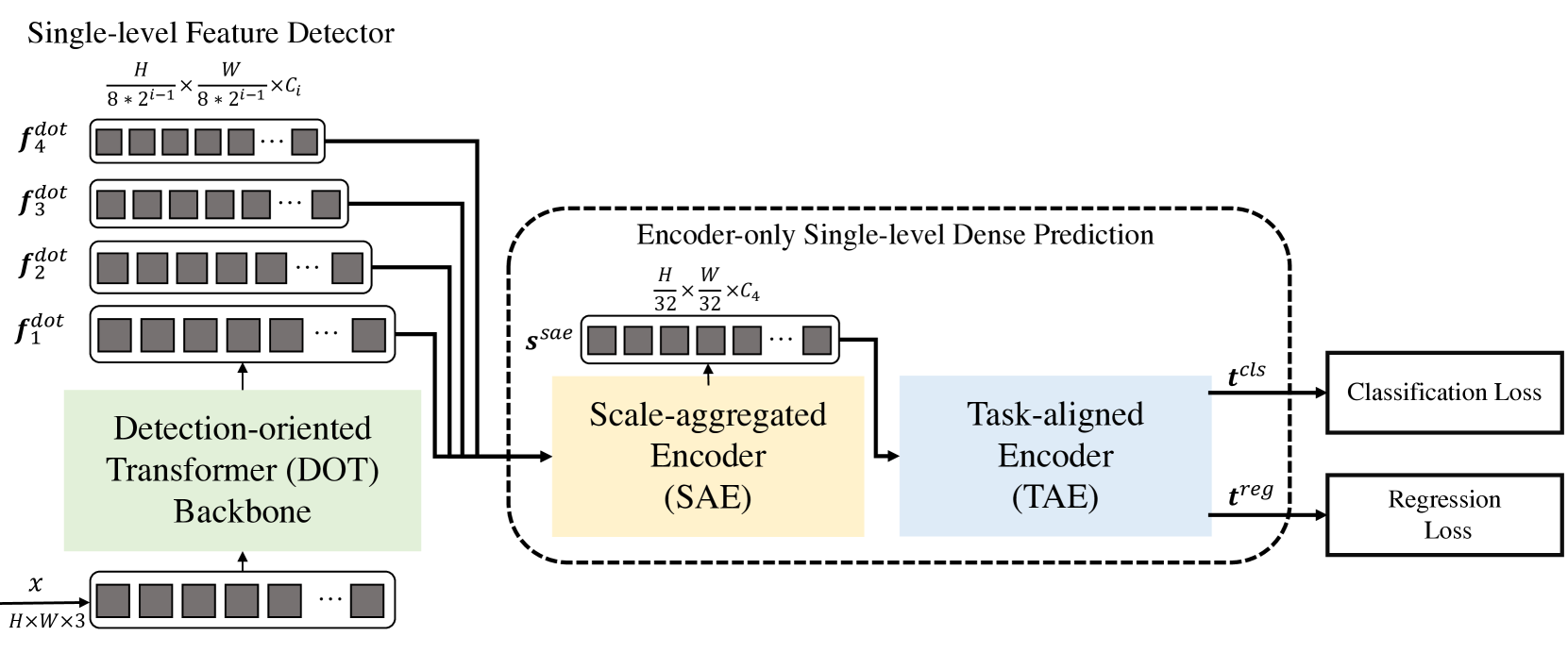
The Decoder-Free Fully Transformer-based (DFFT) method is an efficient object detector based entirely on Decoder-free Transformers. The Transformer backbone is focused on object detection. It extracts them at four scales and sends them to the next single-level encoder-only density prediction module. The prediction module first aggregates the multi-scale feature into a single feature map using the Scale-Aggregated Encoder.
Then, the authors of the method suggest using the Task-Aligned Encoder for simultaneous feature matching for classification and regression problems.
Detection-Oriented Transformer (DOT) backbone is designed to extract multi-scale features with strict semantics. It hierarchically stacks one Embedding module and four DOT stages. The new semantically enhanced attention module aggregates the low-level semantic information of each two successive stages of DOT.
When processing high-resolution feature maps for dense prediction, conventional transformer blocks reduce computational costs by replacing the multi-head Self-Attention (MSA) with the layer of local spatial attention and a biased windowed multi-head Self-Attention (SW-MSA). However, this structure reduces detection performance because it only extracts multi-scale objects with limited low-level semantics.
To mitigate this drawback, the authors of the DFFT method added to the DOT block several SW-MSA blocks and one global attention block across channels. Note that each attention block contains an attention layer and an FFN layer.
The authors of the method found that placing a light attention layer on channels after successive local spatial attention layers can help infer the semantics of an object at each scale.
While the DOT block improves the semantic information in low-level features through global attention across channels, the semantics can be improved further to improve the detection task. For this purpose, the authors of the method propose a new module of Semantic-Augmented Attention (SAA), which exchanges semantic information between two successive DOT layers and complements their features. SAA consists of an upsampling layer and a global attention block across channels. The authors of the method add SAA to every two consecutive DOT blocks. Formally, SAA accepts the results of the current DOT block and the previous-stage DOT, and then returns a semantic-augmented function, which is sent to the next DOT stage and also contributes to the final multi-scale features.
In general, the detection-oriented stage consists of four DOT layers, where each stage includes one DOT block and one SAA module (except for the first stage). In particular, the first stage contains one DOT block and does not contain a SAA module, since the SAA module inputs come from two successive DOT stages. Next comes a downsampling layer to reconstruct the input dimension.
The following module is designed to improve the efficiency of both inference and model training efficiency DFFT. First, it uses a Scale-Aggregated Encoder (SAE) for aggregating multi-scale objects from the DOT backbone into one Ssae object map.
Then it uses the Task-Aligned Encoder (TAE) to create an aligned classification function 𝒕cls and regression function 𝒕reg simultaneously in one head.
The aggregated scale encoder is built from 3 SAE blocks. Each SAE block takes two objects as input data and aggregates them step by step across all SAE blocks. The authors of the method use the scale of finite aggregation of objects to balance detection accuracy and computational costs.
Typically, detectors perform object classification and localization independently of each other using two separate branches (unconnected heads). This two-branch structure does not take into account the interaction between the two tasks and leads to inconsistent predictions. Meanwhile, when learning features for two tasks, there are usually conflicts in the conjugate head. The authors of the DFFT method propose using a task-specific encoder that provides a better balance between learning interactive and task-specific features by combining group attentional units across channels in a connected head.
This encoder consists of two kinds of channel attention blocks. First, multi-level group attention blocks across channels align and separate Ssae aggregated objects into 2 parts. Second, global attention blocks across channels encode one of the two separated objects for the subsequent regression task.
In particular, the differences between the group block of channel attention and the global block of channel attention are that all linear projections, with the exception of projections for Query/Key/Value embeddings in a group attention block across channels, are performed in two groups. Thus, features interact in attention operations while being output separately in output projections.
The original visualization of the method presented by the paper authors is provided below.
2. Implementation using MQL5
After considering the theoretical aspects of the Decoder-Free Fully Transformer-based (DFFT) method, let's move on to implementing the proposed approaches using MQL5. However, our model will be slightly different from the original method. When building the model, we take into account the differences in the specifics of computer vision problems for which the method was proposed, and operations in financial markets for which we are building our model.
2.1 DOT block construction
Before we start, please note that the proposed approaches are quite different from the models we built earlier. The DOT block also differs from the attention blocks we examined earlier. Therefore, we begin our work by building a new neural layer CNeuronDOTOCL. We create our new layer as a descendant of CNeuronBaseOCL, our base class of neural layers.
Similar to other attention blocks, we will add variables to store key parameters:
- iWindowSize — window size of one sequence element;
- iPrevWindowSize — window size of one element of the previous layer sequence;
- iDimension — size of the vector of internal entities Query, Key and Value;
- iUnits — number of elements in the sequence;
- iHeads — number of attention heads.
I think you noticed the variable iPrevWindowSize. The addition of this variable will allow us to implement the ability to compress data from layer to layer, as provided by the DFFT method.
Also, in order to minimize work directly in the new class and maximize the use of previously created developments, we implement part of the functionality using nested neural layers from our library. We will consider their functionality in detail while implementing feed-forward and back-propagation methods.
class CNeuronDOTOCL     :  public CNeuronBaseOCL
  {
protected:
   uint              iWindowSize;
   uint              iPrevWindowSize;
   uint              iDimension;
   uint              iUnits;
   uint              iHeads;
   //---
   CNeuronConvOCL    cProjInput;
   CNeuronConvOCL    cQKV;
   int               iScoreBuffer;
   CNeuronBaseOCL    cRelativePositionsBias;
   CNeuronBaseOCL    MHAttentionOut;
   CNeuronConvOCL    cProj;
   CNeuronBaseOCL    AttentionOut;
   CNeuronConvOCL    cFF1;
   CNeuronConvOCL    cFF2;
   CNeuronBaseOCL    SAttenOut;
   CNeuronXCiTOCL    cCAtten;
   //---
   virtual bool      feedForward(CNeuronBaseOCL *NeuronOCL);
   virtual bool      DOT(void);
   //---
   virtual bool      updateInputWeights(CNeuronBaseOCL *NeuronOCL);
   virtual bool      updateRelativePositionsBias(void);
   virtual bool      DOTInsideGradients(void);

public:
                     CNeuronDOTOCL(void) {};
                    ~CNeuronDOTOCL(void) {};
   //---
   virtual bool      Init(uint numOutputs, uint myIndex, COpenCLMy *open_cl,
                          uint window, uint dimension, uint heads,
                          uint units_count, uint prev_window,
                          ENUM_OPTIMIZATION optimization_type,
                          uint batch);
   virtual bool      calcInputGradients(CNeuronBaseOCL *prevLayer);
   //---
   virtual int       Type(void)   const   {  return defNeuronDOTOCL;   }
   //--- methods for working with files
   virtual bool      Save(int const file_handle);
   virtual bool      Load(int const file_handle);
   virtual CLayerDescription* GetLayerInfo(void);
   virtual bool      WeightsUpdate(CNeuronBaseOCL *source, float tau);
   virtual void      SetOpenCL(COpenCLMy *obj);
  };
In general, the list of overridden methods is standard.
In the class body, we use static objects. This allows us to leave the class constructor and destructor empty.
The class is initialized in the Init method. The necessary data is passed to the method in the parameters. The minimum necessary control of the information is implemented in the relevant method of the parent class. Here we also initialize inherited objects.
bool CNeuronDOTOCL::Init(uint numOutputs, uint myIndex, COpenCLMy *open_cl, uint window,
                         uint dimension, uint heads, uint units_count, uint prev_window,
                         ENUM_OPTIMIZATION optimization_type, uint batch)
  {
//---
   if(!CNeuronBaseOCL::Init(numOutputs, myIndex, open_cl, window * units_count,
                                                      optimization_type, batch))
      return false;
Then we check whether the size of the source data matches the parameters of the current layer. If necessary, initialize the data scaling layer.
   if(prev_window != window)
     {
      if(!cProjInput.Init(0, 0, OpenCL, prev_window, prev_window, window, units_count,
                                                              optimization_type, batch))
         return false;
     }
Next, we save the basic constants received from the caller, which define the architecture of the layer into internal class variables.
   iWindowSize = window;
   iPrevWindowSize = prev_window;
   iDimension = dimension;
   iHeads = heads;
   iUnits = units_count;
Then we sequentially initialize all internal objects. First, we initialize the layer where we generate the Query, Key and Value layers. We will generate all the 3 entities in parallel in the body of one neural layer cQKV.
   if(!cQKV.Init(0, 1, OpenCL, window, window, dimension * heads, units_count,
                                                      optimization_type, batch))
      return false;
Next, we will create the iScoreBuffer buffer for recording object dependency coefficients. It should be noted here that in the DOT block, we first analyze the local semantics. To do this, we check the dependency between an object and its 2 nearest neighbors. Therefore, we define the Score buffer size as iUnits * iHeads * 3.
In addition, the coefficients stored in the buffer are recalculated with each feed-forward pass. They are used only on the next backpropagation pass. Therefore, we will not save the buffer data to the model save file. Moreover, we will not even create a buffer in the main program's memory. We just need to create a buffer in the OpenCL context memory. On the main program side, we will only store a pointer to the buffer.
//---
   iScoreBuffer = OpenCL.AddBuffer(sizeof(float) * iUnits * iHeads * 3, CL_MEM_READ_WRITE);
   if(iScoreBuffer < 0)
      return false;
In the windowed Self-Attention mechanism, unlike the classic transformer, each token interacts only with tokens within a specific window. This significantly reduces computational complexity. However, this limitation also means that models must take into account the relative positions of tokens within the window. To implement this functionality, we introduce trainable parameters cRelativePositionsBias. For each pair of tokens (i, j) inside the iWindowSize window, cRelativePositionsBias contains a weight that determines the importance of the interaction between these tokens based on their relative positions.
The size of this buffer is equal to the size of the Score coefficient buffer. However, to train parameters, in addition to the buffer of the values themselves, we will need additional buffers. In order to reduce the number of internal objects and code readability, for cRelativePositionsBias we will declare a neural layer object that contains all the additional buffers.
   if(!cRelativePositionsBias.Init(1, 2, OpenCL, iUnits * iHeads * 3, optimization_type, batch))
      return false;
Similarly, we add the remaining elements of the Self-Attention mechanism.
   if(!MHAttentionOut.Init(0, 3, OpenCL, iUnits * iHeads * iDimension, optimization_type, batch))
      return false;
   if(!cProj.Init(0, 4, OpenCL, iHeads * iDimension, iHeads * iDimension, window, iUnits,
                                                                       optimization_type, batch))
      return false;
   if(!AttentionOut.Init(0, 5, OpenCL, iUnits * window, optimization_type, batch))
      return false;
   if(!cFF1.Init(0, 6, OpenCL, window, window, 4 * window, units_count, optimization_type,batch))
      return false;
   if(!cFF2.Init(0, 7, OpenCL, window * 4, window * 4, window, units_count, optimization_type,
                                                                                          batch))
      return false;
   if(!SAttenOut.Init(0, 8, OpenCL, iUnits * window, optimization_type, batch))
      return false;
As a global block of attention, we use the CNeuronXCiTOCL layer.
   if(!cCAtten.Init(0, 9, OpenCL, window, MathMax(window / 2, 3), 8, iUnits, 1,
                                                       optimization_type, batch))
      return false;
To minimize data copying operations between buffers, we will replace objects and buffers.
   if(!!Output)
      delete Output;
   Output = cCAtten.getOutput();
   if(!!Gradient)
      delete Gradient;
   Gradient = cCAtten.getGradient();
   SAttenOut.SetGradientIndex(cFF2.getGradientIndex());
//---
   return true;
  }
Complete the method execution.
After initializing the class, we move on to building the feed-forward algorithm. Now we move on to organizing the windowed Self-Attention mechanism on the OpenCL program side. For this, we create the DOTFeedForward kernel. In the parameters to the kernel we pass pointers to 4 data buffers:
- qkv — Query, Key and Value entity buffer,
- score — buffer of dependence coefficients,
- rpb — positional offset buffer,
- out — buffer of results of the multi-head windowed Self-Attention.
__kernel void DOTFeedForward(__global float *qkv,
                             __global float *score,
                             __global float *rpb,
                             __global float *out)
  {
   const size_t d = get_local_id(0);
   const size_t dimension = get_local_size(0);
   const size_t u = get_global_id(1);
   const size_t units = get_global_size(1);
   const size_t h = get_global_id(2);
   const size_t heads = get_global_size(2);
We plan to launch the kernel in a 3-dimensional task space. In the body of the kernel, we identify the thread in all 3 dimensions. Here it should be noted that in the first dimension of Query, Key and Value entity dimensions, we create a workgroup with buffer sharing in local memory.
Next, we determine the offsets in the data buffers before the objects being analyzed.
   uint step = 3 * dimension * heads;
   uint start = max((int)u - 1, 0);
   uint stop = min((int)u + 1, (int)units - 1);
   uint shift_q = u * step + h * dimension;
   uint shift_k = start * step + dimension * (heads + h);
   uint shift_score = u * 3 * heads;
We also create here a local buffer for data exchange between threads of the same workgroup.
   const uint ls_d = min((uint)dimension, (uint)LOCAL_ARRAY_SIZE);
   __local float temp[LOCAL_ARRAY_SIZE][3];
As mentioned earlier, we determine local semantics by the 2 nearest neighbors of an object. First, we determine the influence of neighbors on the analyzed object. We calculate the dependence coefficients within the working group. First we multiply the elements of entities Query and Key in pairs, in parallel streams.
//--- Score
   if(d < ls_d)
     {
      for(uint pos = start; pos <= stop; pos++)
        {
         temp[d][pos - start] = 0;
        }
      for(uint dim = d; dim < dimension; dim += ls_d)
        {
         float q = qkv[shift_q + dim];
         for(uint pos = start; pos <= stop; pos++)
           {
            uint i = pos - start;
            temp[d][i] = temp[d][i] + q * qkv[shift_k + i * step + dim];
           }
        }
      barrier(CLK_LOCAL_MEM_FENCE);
Then we summarize the resulting products.
      int count = ls_d;
      do
        {
         count = (count + 1) / 2;
         if(d < count && (d + count) < dimension)
            for(uint i = 0; i <= (stop - start); i++)
              {
               temp[d][i] += temp[d + count][i];
               temp[d + count][i] = 0;
              }
         barrier(CLK_LOCAL_MEM_FENCE);
        }
      while(count > 1);
     }
We add offset parameters to the obtained values and normalize with the SoftMax function.
   if(d == 0)
     {
      float sum = 0;
      for(uint i = 0; i <= (stop - start); i++)
        {
         temp[0][i] = exp(temp[0][i] + rpb[shift_score + i]);
         sum += temp[0][i];
        }
      for(uint i = 0; i <= (stop - start); i++)
        {
         temp[0][i] = temp[0][i] / sum;
         score[shift_score + i] = temp[0][i];
        }
     }
   barrier(CLK_LOCAL_MEM_FENCE);
The result is saved in the dependency coefficient buffer.
Now we can multiply the resulting coefficients by the corresponding elements of the Value entity to determine the results of a multi-headed windowed Self-Attention block.
   int shift_out = dimension * (u * heads + h) + d;
   int shift_v = dimension * (heads * (u * 3 + 2) + h);
   float sum = 0;
   for(uint i = 0; i <= (stop - start); i++)
      sum += qkv[shift_v + i] * temp[0][i];
   out[shift_out] = sum;
  }
We save the resulting values into the corresponding elements of the results buffer and terminate the kernel.
After creating the kernel, we return to our main program, where we create the methods of our new CNeuronDOTOCL class. First, we create the DOT method, in which the above created kernel is placed in the execution queue.
The method algorithm is quite simple. We simply pass external parameters to the kernel.
bool CNeuronDOTOCL::DOT(void)
  {
   if(!OpenCL)
      return false;
//---
   uint global_work_offset[3] = {0, 0, 0};
   uint global_work_size[3] = {iDimension, iUnits, iHeads};
   uint local_work_size[3] = {iDimension, 1, 1};
   if(!OpenCL.SetArgumentBuffer(def_k_DOTFeedForward, def_k_dot_qkv, cQKV.getOutputIndex()))
      return false;
   if(!OpenCL.SetArgumentBuffer(def_k_DOTFeedForward, def_k_dot_score, iScoreBuffer))
      return false;
   if(!OpenCL.SetArgumentBuffer(def_k_DOTFeedForward, def_k_dot_rpb,
                                                    cRelativePositionsBias.getOutputIndex()))
      return false;
   if(!OpenCL.SetArgumentBuffer(def_k_DOTFeedForward, def_k_dot_out,
                                                            MHAttentionOut.getOutputIndex()))
      return false;
Then we send the kernel to the execution queue.
   ResetLastError();
   if(!OpenCL.Execute(def_k_DOTFeedForward, 3, global_work_offset, global_work_size,
                                                                     local_work_size))
     {
      printf("Error of execution kernel %s: %d", __FUNCTION__, GetLastError());
      return false;
     }
//---
   return true;
  }
Do not forget to control the results at each step.
After completing the preparatory work, we move on to creating the CNeuronDOTOCL::feedForward method, in which we will define the feed-forward algorithm for our layer.
In the method parameters we receive a pointer to the layer of the previous neural layer. For ease of use, let's save the resulting pointer into a local variable.
bool CNeuronDOTOCL::feedForward(CNeuronBaseOCL *NeuronOCL)
  {
   CNeuronBaseOCL* inputs = NeuronOCL;
Next, we check whether the size of the source data differs from the parameters of the current layer. If necessary, we scale the source data and calculate Query, Key and Value entities.
In case of equality of data buffers, we omit the scaling step and immediately generate the Query, Key and Value entities.
   if(iPrevWindowSize != iWindowSize)
     {
      if(!cProjInput.FeedForward(inputs) ||
         !cQKV.FeedForward(GetPointer(cProjInput)))
         return false;
      inputs = GetPointer(cProjInput);
     }
   else
      if(!cQKV.FeedForward(inputs))
         return false;
The next step is to call the above created windowed Self-Attention method.
   if(!DOT())
      return false;
Reducing the data dimension.
   if(!cProj.FeedForward(GetPointer(MHAttentionOut)))
      return false;
Adding the result with the source data buffer.
   if(!SumAndNormilize(inputs.getOutput(), cProj.getOutput(), AttentionOut.getOutput(),
                                                                     iWindowSize, true))
      return false;
Propagating the result through the FeedForward block.
   if(!cFF1.FeedForward(GetPointer(AttentionOut)))
      return false;
   if(!cFF2.FeedForward(GetPointer(cFF1)))
      return false;
Adding the buffer results again. This time we add the results with the output of the windowed Self-Attention block.
   if(!SumAndNormilize(AttentionOut.getOutput(), cFF2.getOutput(), SAttenOut.getOutput(),
                                                                        iWindowSize, true))
      return false;
At the end of the block there is the global Self-Attention. For this stage, we use the CNeuronXCiTOCL layer.
   if(!cCAtten.FeedForward(GetPointer(SAttenOut)))
      return false;
//---
   return true;
  }
We check the results of the operations and terminate the method.
This concludes our consideration of the implementation of the feed-forward pass of our class. Next, we move on to implementing the backpropagation methods. Here we also start work by creating a backpropagation kernel of the windowed Self-Attention block: DOTInsideGradients. Like the feed-forward kernel, we launch the new kernel in a 3-dimensional task space. However, this time we do not create local groups.
In the parameters, the kernel receives pointers to all necessary data buffers.
__kernel void DOTInsideGradients(__global float *qkv, __global float *qkv_g,
                                 __global float *scores,
                                 __global float *rpb, __global float *rpb_g,
                                 __global float *gradient)
  {
//--- init
   const uint u = get_global_id(0);
   const uint d = get_global_id(1);
   const uint h = get_global_id(2);
   const uint units = get_global_size(0);
   const uint dimension = get_global_size(1);
   const uint heads = get_global_size(2);
In the body of the kernel, we identify the thread in all 3 dimensions. We also determine the task space, which will indicate the size of the resulting buffers.
Here we also determine the offset in the data buffers.
   uint step = 3 * dimension * heads;
   uint start = max((int)u - 1, 0);
   uint stop = min((int)u + 1, (int)units - 1);
   const uint shift_q = u * step + dimension * h + d;
   const uint shift_k = u * step + dimension * (heads + h) + d;
   const uint shift_v = u * step + dimension * (2 * heads + h) + d;
Then we move directly to the gradient distribution. First, we define the error gradient for the Value element. To do this, we multiply the resulting gradient by the corresponding influence coefficient.
//--- Calculating Value's gradients
   float sum = 0;
   for(uint i = start; i <= stop; i ++)
     {
      int shift_score = i * 3 * heads;
      if(u == i)
        {
         shift_score += (uint)(u > 0);
        }
      else
        {
         if(u > i)
            shift_score += (uint)(start > 0) + 1;
        }
      uint shift_g = dimension * (i * heads + h) + d;
      sum += gradient[shift_g] * scores[shift_score];
     }
   qkv_g[shift_v] = sum;
The next step is to define the error gradient for the Query entity. Here the algorithm is a little more complicated. We first need to determine the error gradient for the corresponding vector of dependency coefficients and adjust the resulting gradient to the derivative of the SoftMax function. Only after this we can multiply the resulting error gradient of the dependence coefficients by the corresponding element of the Key entity tensor.
Please note that before normalizing the dependence coefficients, we added them with elements of the positional attentional bias. As you know, when adding, we transfer the gradient in full in both directions. Double counting of errors is easily offset by a small learning coefficient. Therefore, we transfer the error gradient at the level of the dependence coefficient matrix to the positional shift error gradient buffer.
//--- Calculating Query's gradients
   float grad = 0;
   uint shift_score = u * heads * 3;
   for(int k = start; k <= stop; k++)
     {
      float sc_g = 0;
      float sc = scores[shift_score + k - start];
      for(int v = start; v <= stop; v++)
         for(int dim=0;dim<dimension;dim++)
            sc_g += scores[shift_score + v - start] *
                    qkv[v * step + dimension * (2 * heads + h) + dim] *
                    gradient[dimension * (u * heads + h) + dim] *
                    ((float)(k == v) - sc);
      grad += sc_g * qkv[k * step + dimension * (heads + h) + d];
      if(d == 0)
         rpb_g[shift_score + k - start] = sc_g;
     }
   qkv_g[shift_q] = grad;
Next, we just need to define the error gradient for the Key entity in a similar way. The algorithm is similar to Query, but it has a different dimension of the coefficient matrix.
//--- Calculating Key's gradients
   grad = 0;
   for(int q = start; q <= stop; q++)
     {
      float sc_g = 0;
      shift_score = q * heads * 3;
      if(u == q)
        {
         shift_score += (uint)(u > 0);
        }
      else
        {
         if(u > q)
            shift_score += (uint)(start > 0) + 1;
        }
      float sc = scores[shift_score];
      for(int v = start; v <= stop; v++)
        {
         shift_score = v * heads * 3;
         if(u == v)
           {
            shift_score += (uint)(u > 0);
           }
         else
           {
            if(u > v)
               shift_score += (uint)(start > 0) + 1;
           }
         for(int dim=0;dim<dimension;dim++)
            sc_g += scores[shift_score] * qkv[shift_v-d+dim] *
                    gradient[dimension * (v * heads + h) + d] * ((float)(d == v) - sc);
        }
      grad += sc_g * qkv[q * step + dimension * h + d];
     }
   qkv_g[shift_k] = grad;
  }
With this we finish working with the kernel and return to working with our CNeuronDOTOCL class, in which we will create the DOTInsideGradients method to call the above created kernel. The algorithm remains the same:
- Defining the task space
bool CNeuronDOTOCL::DOTInsideGradients(void)
  {
   if(!OpenCL)
      return false;
//---
   uint global_work_offset[3] = {0, 0, 0};
   uint global_work_size[3] = {iUnits, iDimension, iHeads};
- Passing the parameters
   if(!OpenCL.SetArgumentBuffer(def_k_DOTInsideGradients, def_k_dotg_qkv,
                                                                   cQKV.getOutputIndex()))
      return false;
   if(!OpenCL.SetArgumentBuffer(def_k_DOTInsideGradients, def_k_dotg_qkv_g,
                                                                  cQKV.getGradientIndex()))
      return false;
   if(!OpenCL.SetArgumentBuffer(def_k_DOTInsideGradients, def_k_dotg_scores, iScoreBuffer))
      return false;
   if(!OpenCL.SetArgumentBuffer(def_k_DOTInsideGradients, def_k_dotg_rpb,
                                                  cRelativePositionsBias.getOutputIndex()))
      return false;
   if(!OpenCL.SetArgumentBuffer(def_k_DOTInsideGradients, def_k_dotg_rpb_g,
                                                cRelativePositionsBias.getGradientIndex()))
      return false;
   if(!OpenCL.SetArgumentBuffer(def_k_DOTInsideGradients, def_k_dotg_gradient,
                                                        MHAttentionOut.getGradientIndex()))
      return false;
- Putting in the execution queue
   ResetLastError();
   if(!OpenCL.Execute(def_k_DOTInsideGradients, 3, global_work_offset, global_work_size))
     {
      printf("Error of execution kernel %s: %d", __FUNCTION__, GetLastError());
      return false;
     }
//---
   return true;
  }
- Then we check the result of the operations and terminate the method.
We describe the backpropagation pass algorithm directly in the calcInputGradients method. In the parameters, the method receives a pointer to the object of the previous layer to which the error should be propagated. In the body of the method, we immediately check the relevance of the received pointer. Because if the pointer is invalid, we have nowhere to pass the error gradient. Then the logical meaning of all operations would be close to "0".
bool CNeuronDOTOCL::calcInputGradients(CNeuronBaseOCL *prevLayer)
  {
   if(!prevLayer)
      return false;
Next, we repeat the feed-forward pass operations in reverse order. When initializing our CNeuronDOTOCL class, we prudently replaced the buffers. Now, when receiving the error gradient from the subsequent neural layer, we received it directly into the global attention layer. Consequently, we omit the already unnecessary data copying operation and immediately call the relevant method in the internal layer of global attention.
   if(!cCAtten.calcInputGradients(GetPointer(SAttenOut)))
      return false;
Here we also used the buffer substitution technique and immediately propagated the error gradient through the FeedForward block.
   if(!cFF2.calcInputGradients(GetPointer(cFF1)))
      return false;
   if(!cFF1.calcInputGradients(GetPointer(AttentionOut)))
      return false;
Next, we sum the error gradient from the 2 threads.
   if(!SumAndNormilize(AttentionOut.getGradient(), SAttenOut.getGradient(),
                                   cProj.getGradient(), iWindowSize, false))
      return false;
Then we distribute it among the attention heads.
   if(!cProj.calcInputGradients(GetPointer(MHAttentionOut)))
      return false;
Calling our method for distributing the error gradient through the windowed Self-Attention block.
   if(!DOTInsideGradients())
      return false;
Then we check the size of the previous and current layers. If we need to scale data, we first propagate the error gradient onto the scaling layer. We sum up the error gradients from 2 threads. Only then we scale the error gradient to the previous layer.
   if(iPrevWindowSize != iWindowSize)
     {
      if(!cQKV.calcInputGradients(GetPointer(cProjInput)))
         return false;
      if(!SumAndNormilize(cProjInput.getGradient(), cProj.getGradient(),
                          cProjInput.getGradient(), iWindowSize, false))
         return false;
      if(!cProjInput.calcInputGradients(prevLayer))
         return false;
     }
If the neural layers are equal, we immediately transfer the error gradient to the previous layer. Then we supplement it with the error gradient from the second thread.
   else
     {
      if(!cQKV.calcInputGradients(prevLayer))
         return false;
      if(!SumAndNormilize(prevLayer.getGradient(), cProj.getGradient(),
                          prevLayer.getGradient(), iWindowSize, false))
         return false;
     }
//---
   return true;
  }
After propagating the error gradient through all neural layers, we need to update the model parameters to minimize the error. Everything would be simple here if not for one thing. Remember the element positional influence parameter buffer? We need to update its parameters. To perform this functionality, we create the RPBUpdateAdam kernel. In the parameters to the kernel, we pass pointers to the buffer of current parameters and the error gradient. We also pass auxiliary tensors and constants of the Adam method.
__kernel void RPBUpdateAdam(__global float *target,
                             __global const float *gradient,
                             __global float *matrix_m,   ///<[in,out] Matrix of first momentum
                             __global float *matrix_v,   ///<[in,out] Matrix of seconfd momentum
                             const float b1,             ///< First momentum multiplier
                             const float b2              ///< Second momentum multiplier
                            )
  {
   const int i = get_global_id(0);
In the body of the kernel, we identify a thread, which indicates the offset in the data buffers.
Next, we declare local variables and save the necessary values of global buffers in them.
   float m, v, weight;
   m = matrix_m[i];
   v = matrix_v[i];
   weight = target[i];
   float g = gradient[i];
In accordance with the Adam method, we first determine the momentums.
   m = b1 * m + (1 - b1) * g;
   v = b2 * v + (1 - b2) * pow(g, 2);
Based on the obtained momentums, will calculate the necessary adjustment of the parameter.
float delta = m / (v != 0.0f ? sqrt(v) : 1.0f);
We save all the data to the corresponding elements of global buffers.
   target[i] = clamp(weight + delta, -MAX_WEIGHT, MAX_WEIGHT);
   matrix_m[i] = m;
   matrix_v[i] = v;
  }
Let's return to our CNeuronDOTOCL class and create the updateRelativePositionsBias method that calls the kernel. Here we use a 1-dimensional task space.
bool CNeuronDOTOCL::updateRelativePositionsBias(void)
  {
   if(!OpenCL)
      return false;
//---
   uint global_work_offset[1] = {0};
   uint global_work_size[1] = {cRelativePositionsBias.Neurons()};
   if(!OpenCL.SetArgumentBuffer(def_k_RPBUpdateAdam, def_k_rpbw_rpb,
                                         cRelativePositionsBias.getOutputIndex()))
      return false;
   if(!OpenCL.SetArgumentBuffer(def_k_RPBUpdateAdam, def_k_rpbw_gradient,
                                         cRelativePositionsBias.getGradientIndex()))
      return false;
   if(!OpenCL.SetArgumentBuffer(def_k_RPBUpdateAdam, def_k_rpbw_matrix_m,
                                    cRelativePositionsBias.getFirstMomentumIndex()))
      return false;
   if(!OpenCL.SetArgumentBuffer(def_k_RPBUpdateAdam, def_k_rpbw_matrix_v,
                                   cRelativePositionsBias.getSecondMomentumIndex()))
      return false;
   if(!OpenCL.SetArgument(def_k_RPBUpdateAdam, def_k_rpbw_b1, b1))
      return false;
   if(!OpenCL.SetArgument(def_k_RPBUpdateAdam, def_k_rpbw_b2, b2))
      return false;
   ResetLastError();
   if(!OpenCL.Execute(def_k_RPBUpdateAdam, 1, global_work_offset, global_work_size))
     {
      printf("Error of execution kernel %s: %d", __FUNCTION__, GetLastError());
      return false;
     }
//---
   return true;
  }
The preparatory work has been completed. Next, we move on to creating the top-level method updateInputWeights for updating block parameters. In the parameters, the method receives a pointer to the object of the previous layer. In this case, we omit checking the received pointer, since the check will be performed in the methods of the internal layers.
First we check whether the scaling layer parameters need to be updated. If necessary the update is required, we call the relevant method on the specified layer.
   if(iWindowSize != iPrevWindowSize)
     {
      if(!cProjInput.UpdateInputWeights(NeuronOCL))
         return false;
      if(!cQKV.UpdateInputWeights(GetPointer(cProjInput)))
         return false;
     }
   else
     {
      if(!cQKV.UpdateInputWeights(NeuronOCL))
         return false;
     }
Then we update the Query, Key and Value entity generation layer parameters.
Similarly, we update the parameters of all internal layers.
   if(!cProj.UpdateInputWeights(GetPointer(MHAttentionOut)))
      return false;
   if(!cFF1.UpdateInputWeights(GetPointer(AttentionOut)))
      return false;
   if(!cFF2.UpdateInputWeights(GetPointer(cFF1)))
      return false;
   if(!cCAtten.UpdateInputWeights(GetPointer(SAttenOut)))
      return false;
And at the end of the method, we update the positional offset parameters.
   if(!updateRelativePositionsBias())
      return false;
//---
   return true;
  }
Again, we should not forget to control the results at each step.
This concludes our consideration of the methods of the new neural layer CNeuronDOTOCL. You can find the complete code of the class and of its methods, including those not described in this article, in the attachment.
We move on and proceed to build the architecture of our new model.
2.2 Model architecture
As usual, we will describe the architecture of our model in the CreateDescriptions method. In the parameters, the method receives pointers to 3 dynamic arrays for storing model descriptions. In the body of the method, we immediately check the relevance of the received pointers and, if necessary, create new instances of the arrays.
bool CreateDescriptions(CArrayObj *dot, CArrayObj *actor, CArrayObj *critic)
  {
//---
   CLayerDescription *descr;
//---
   if(!dot)
     {
      dot = new CArrayObj();
      if(!dot)
         return false;
     }
   if(!actor)
     {
      actor = new CArrayObj();
      if(!actor)
         return false;
     }
   if(!critic)
     {
      critic = new CArrayObj();
      if(!critic)
         return false;
     }
We need to create 3 models:
- DOT
- Actor
- Critic.
The DOT block is provided by the DFFT architecture. However, there is nothing about the Actor or the Critic. But I want to remind you that the DFFT method suggests the creation of a TAE block with classification and regression outputs. Consecutive use of Actor and Critic should emit the TAE block. The Actor is the action classifier, and the Critic is the reward regression.
We feed the DOT model a description of the current state of the environment.
//--- DOT
   dot.Clear();
//--- Input layer
   if(!(descr = new CLayerDescription()))
      return false;
   descr.type = defNeuronBaseOCL;
   int prev_count = descr.count = (HistoryBars * BarDescr);
   descr.activation = None;
   descr.optimization = ADAM;
   if(!dot.Add(descr))
     {
      delete descr;
      return false;
     }
We process the "raw" data in the batch normalization layer.
//--- layer 1
   if(!(descr = new CLayerDescription()))
      return false;
   descr.type = defNeuronBatchNormOCL;
   descr.count = prev_count;
   descr.batch = MathMax(1000, GPTBars);
   descr.activation = None;
   descr.optimization = ADAM;
   if(!dot.Add(descr))
     {
      delete descr;
      return false;
     }
Then we create an embedding of the latest data and add it to the stack.
   if(!(descr = new CLayerDescription()))
      return false;
   descr.type = defNeuronEmbeddingOCL;
     {
      int temp[] = {prev_count};
      ArrayCopy(descr.windows, temp);
     }
   prev_count = descr.count = GPTBars;
   int prev_wout = descr.window_out = EmbeddingSize;
   if(!dot.Add(descr))
     {
      delete descr;
      return false;
     }
Next we add positional encoding of the data.
//--- layer 3
   if(!(descr = new CLayerDescription()))
      return false;
   descr.type = defNeuronPEOCL;
   descr.count = prev_count;
   descr.window = prev_wout;
   if(!dot.Add(descr))
     {
      delete descr;
      return false;
     }
Up to this point, we have repeated the embedding architecture from previous works. Then we have changes. We add the first DOT block, in which analysis is implemented in the context of individual states.
//--- layer 4
   if(!(descr = new CLayerDescription()))
      return false;
   descr.type = defNeuronDOTOCL;
   descr.count = prev_count;
   descr.window = prev_wout;
   descr.step  =  4;
   descr.window_out = prev_wout / descr.step;
   if(!dot.Add(descr))
     {
      delete descr;
      return false;
     }
In the next block, we compress the data by two times but continue to analyze in the context of individual states.
//--- layer 5
   if(!(descr = new CLayerDescription()))
      return false;
   descr.type = defNeuronDOTOCL;
   descr.count = prev_count;
   prev_wout = descr.window = prev_wout / 2;
   descr.step  =  4;
   descr.window_out = prev_wout / descr.step;
   if(!dot.Add(descr))
     {
      delete descr;
      return false;
     }
Next, we group the data for analysis into 2 sequential states.
//--- layer 6
   if(!(descr = new CLayerDescription()))
      return false;
   descr.type = defNeuronDOTOCL;
   prev_count = descr.count = prev_count / 2;
   prev_wout = descr.window = prev_wout * 2;
   descr.step  =  4;
   descr.window_out = prev_wout / descr.step;
   if(!dot.Add(descr))
     {
      delete descr;
      return false;
     }
Once again we compress the data.
//--- layer 7
   if(!(descr = new CLayerDescription()))
      return false;
   descr.type = defNeuronDOTOCL;
   descr.count = prev_count;
   prev_wout = descr.window = prev_wout / 2;
   descr.step  =  4;
   descr.window_out = prev_wout / descr.step;
   if(!dot.Add(descr))
     {
      delete descr;
      return false;
     }
The last layer of the DOT model goes beyond the DFFT method. Here I added a cross-attention layer.
//--- layer 8
   if(!(descr = new CLayerDescription()))
      return false;
   descr.type = defNeuronMH2AttentionOCL;
   descr.count = prev_wout;
   descr.window = prev_count;
   descr.step = 4;
   descr.window_out = prev_wout / descr.step;
   descr.optimization = ADAM;
   if(!dot.Add(descr))
     {
      delete descr;
      return false;
     }
The Actor model receives input processed in the DOT model of the environmental state.
//--- Actor
   actor.Clear();
//--- Input layer
   if(!(descr = new CLayerDescription()))
      return false;
   descr.type = defNeuronBaseOCL;
   descr.count = prev_count*prev_wout;
   descr.activation = None;
   descr.optimization = ADAM;
   if(!actor.Add(descr))
     {
      delete descr;
      return false;
     }
The received data is combined with the current account status.
//--- layer 1
   if(!(descr = new CLayerDescription()))
      return false;
   descr.type = defNeuronConcatenate;
   descr.count = LatentCount;
   descr.window = prev_count * prev_wout;
   descr.step = AccountDescr;
   descr.optimization = ADAM;
   descr.activation = SIGMOID;
   if(!actor.Add(descr))
     {
      delete descr;
      return false;
     }
Data is processed by 2 fully connected layers.
//--- layer 2
   if(!(descr = new CLayerDescription()))
      return false;
   descr.type = defNeuronBaseOCL;
   descr.count = LatentCount;
   descr.activation = SIGMOID;
   descr.optimization = ADAM;
   if(!actor.Add(descr))
     {
      delete descr;
      return false;
     }
//--- layer 3
   if(!(descr = new CLayerDescription()))
      return false;
   descr.type = defNeuronBaseOCL;
   descr.count = 2 * NActions;
   descr.activation = None;
   descr.optimization = ADAM;
   if(!actor.Add(descr))
     {
      delete descr;
      return false;
     }
At the output we generate a stochastic Actor policy.
//--- layer 4
   if(!(descr = new CLayerDescription()))
      return false;
   descr.type = defNeuronVAEOCL;
   descr.count = NActions;
   descr.optimization = ADAM;
   if(!actor.Add(descr))
     {
      delete descr;
      return false;
     }
The Critic also uses processed environmental states as input.
//--- Critic
   critic.Clear();
//--- Input layer
   if(!(descr = new CLayerDescription()))
      return false;
   descr.Copy(actor.At(0));
   if(!critic.Add(descr))
     {
      delete descr;
      return false;
     }
We supplement the description of the environmental state with the actions of the Agent.
//--- layer 1
   if(!(descr = new CLayerDescription()))
      return false;
   descr.Copy(actor.At(0));
   descr.step = NActions;
   descr.optimization = ADAM;
   descr.activation = SIGMOID;
   if(!critic.Add(descr))
     {
      delete descr;
      return false;
     }
The data is processed by 2 fully connected layers with a reward vector at the output.
//--- layer 2
   if(!(descr = new CLayerDescription()))
      return false;
   descr.type = defNeuronBaseOCL;
   descr.count = LatentCount;
   descr.activation = SIGMOID;
   descr.optimization = ADAM;
   if(!critic.Add(descr))
     {
      delete descr;
      return false;
     }
//--- layer 3
   if(!(descr = new CLayerDescription()))
      return false;
   descr.type = defNeuronBaseOCL;
   descr.count = NRewards;
   descr.activation = None;
   descr.optimization = ADAM;
   if(!critic.Add(descr))
     {
      delete descr;
      return false;
     }
//---
   return true;
  }
2.3 Environmental Interaction EA
After creating the architecture of the models, we move on to creating an EA for interaction with the environment "...\Experts\DFFT\Research.mq5". This EA is designed to collect the initial training sample and subsequently update the experience replay buffer. The EA can also be used to test a trained model. Although another EA "...\Experts\DFFT\Test.mq5" is provided to perform this functionality. Both EAs have a similar algorithm. However, the latter does not save data to the experience replay buffer for subsequent training. This is done for a "fair" test of the trained model.
Both EAs are mainly copied from previous works. Within the framework of the article, we will only focus on changes related to the specifics of the models.
While collecting data, we will not use the Critic model.
CNet                 DOT;
CNet                 Actor;
In the EA initialization method, we first connect the necessary indicators.
//+------------------------------------------------------------------+
//| Expert initialization function                                   |
//+------------------------------------------------------------------+
int OnInit()
  {
//---
   if(!Symb.Name(_Symbol))
      return INIT_FAILED;
   Symb.Refresh();
//---
   if(!RSI.Create(Symb.Name(), TimeFrame, RSIPeriod, RSIPrice))
      return INIT_FAILED;
//---
   if(!CCI.Create(Symb.Name(), TimeFrame, CCIPeriod, CCIPrice))
      return INIT_FAILED;
//---
   if(!ATR.Create(Symb.Name(), TimeFrame, ATRPeriod))
      return INIT_FAILED;
//---
   if(!MACD.Create(Symb.Name(), TimeFrame, FastPeriod, SlowPeriod, SignalPeriod, MACDPrice))
      return INIT_FAILED;
   if(!RSI.BufferResize(HistoryBars) || !CCI.BufferResize(HistoryBars) ||
      !ATR.BufferResize(HistoryBars) || !MACD.BufferResize(HistoryBars))
     {
      PrintFormat("%s -> %d", __FUNCTION__, __LINE__);
      return INIT_FAILED;
     }
//---
   if(!Trade.SetTypeFillingBySymbol(Symb.Name()))
      return INIT_FAILED;
//--- load models
   float temp;
Then we try to load pre-trained models.
   if(!DOT.Load(FileName + "DOT.nnw", temp, temp, temp, dtStudied, true) ||
      !Actor.Load(FileName + "Act.nnw", temp, temp, temp, dtStudied, true))
     {
      CArrayObj *dot = new CArrayObj();
      CArrayObj *actor = new CArrayObj();
      CArrayObj *critic = new CArrayObj();
      if(!CreateDescriptions(dot, actor, critic))
        {
         delete dot;
         delete actor;
         delete critic;
         return INIT_FAILED;
        }
      if(!DOT.Create(dot) ||
         !Actor.Create(actor))
        {
         delete dot;
         delete actor;
         delete critic;
         return INIT_FAILED;
        }
      delete dot;
      delete actor;
      delete critic;
     }
If the models could not be loaded, we initialize new models with random parameters. After that we transfer both models into a single OpenCL context.
Actor.SetOpenCL(DOT.GetOpenCL());
We also carry out a minimal check of the model architecture.
   Actor.getResults(Result);
   if(Result.Total() != NActions)
     {
      PrintFormat("The scope of the actor does not match the actions count (%d <> %d)",
                                                               NActions, Result.Total());
      return INIT_FAILED;
     }
//---
   DOT.GetLayerOutput(0, Result);
   if(Result.Total() != (HistoryBars * BarDescr))
     {
      PrintFormat("Input size of Encoder doesn't match state description (%d <> %d)",
                                              Result.Total(), (HistoryBars * BarDescr));
      return INIT_FAILED;
     }
Save the balance state in a local variable.
   PrevBalance = AccountInfoDouble(ACCOUNT_BALANCE);
   PrevEquity = AccountInfoDouble(ACCOUNT_EQUITY);
//---
   return(INIT_SUCCEEDED);
  }
Interaction with the environment and data collection is implemented in the OnTick method. In the method body, we first check the occurrence of a new bar opening event. Any analysis is only performed on a new candle.
//+------------------------------------------------------------------+
//| Expert tick function                                             |
//+------------------------------------------------------------------+
void OnTick()
  {
//---
   if(!IsNewBar())
      return;
Next, we update the historical data.
   int bars = CopyRates(Symb.Name(), TimeFrame, iTime(Symb.Name(), TimeFrame, 1),
                                                               HistoryBars, Rates);
   if(!ArraySetAsSeries(Rates, true))
      return;
//---
   RSI.Refresh();
   CCI.Refresh();
   ATR.Refresh();
   MACD.Refresh();
   Symb.Refresh();
   Symb.RefreshRates();
Fill the buffer for describing the state of the environment.
   float atr = 0;
   for(int b = 0; b < (int)HistoryBars; b++)
     {
      float open = (float)Rates[b].open;
      float rsi = (float)RSI.Main(b);
      float cci = (float)CCI.Main(b);
      atr = (float)ATR.Main(b);
      float macd = (float)MACD.Main(b);
      float sign = (float)MACD.Signal(b);
      if(rsi == EMPTY_VALUE || cci == EMPTY_VALUE || atr == EMPTY_VALUE ||
         macd == EMPTY_VALUE || sign == EMPTY_VALUE)
         continue;
      //---
      int shift = b * BarDescr;
      sState.state[shift] = (float)(Rates[b].close - open);
      sState.state[shift + 1] = (float)(Rates[b].high - open);
      sState.state[shift + 2] = (float)(Rates[b].low - open);
      sState.state[shift + 3] = (float)(Rates[b].tick_volume / 1000.0f);
      sState.state[shift + 4] = rsi;
      sState.state[shift + 5] = cci;
      sState.state[shift + 6] = atr;
      sState.state[shift + 7] = macd;
      sState.state[shift + 8] = sign;
     }
   bState.AssignArray(sState.state);
The next step is to collect data on the current account status.
   sState.account[0] = (float)AccountInfoDouble(ACCOUNT_BALANCE);
   sState.account[1] = (float)AccountInfoDouble(ACCOUNT_EQUITY);
//---
   double buy_value = 0, sell_value = 0, buy_profit = 0, sell_profit = 0;
   double position_discount = 0;
   double multiplyer = 1.0 / (60.0 * 60.0 * 10.0);
   int total = PositionsTotal();
   datetime current = TimeCurrent();
   for(int i = 0; i < total; i++)
     {
      if(PositionGetSymbol(i) != Symb.Name())
         continue;
      double profit = PositionGetDouble(POSITION_PROFIT);
      switch((int)PositionGetInteger(POSITION_TYPE))
        {
         case POSITION_TYPE_BUY:
            buy_value += PositionGetDouble(POSITION_VOLUME);
            buy_profit += profit;
            break;
         case POSITION_TYPE_SELL:
            sell_value += PositionGetDouble(POSITION_VOLUME);
            sell_profit += profit;
            break;
        }
      position_discount += profit - (current - PositionGetInteger(POSITION_TIME)) *
                                     multiplyer * MathAbs(profit);
     }
   sState.account[2] = (float)buy_value;
   sState.account[3] = (float)sell_value;
   sState.account[4] = (float)buy_profit;
   sState.account[5] = (float)sell_profit;
   sState.account[6] = (float)position_discount;
   sState.account[7] = (float)Rates[0].time;
We consolidate the collected data in a buffer describing the account status.
   bAccount.Clear();
   bAccount.Add((float)((sState.account[0] - PrevBalance) / PrevBalance));
   bAccount.Add((float)(sState.account[1] / PrevBalance));
   bAccount.Add((float)((sState.account[1] - PrevEquity) / PrevEquity));
   bAccount.Add(sState.account[2]);
   bAccount.Add(sState.account[3]);
   bAccount.Add((float)(sState.account[4] / PrevBalance));
   bAccount.Add((float)(sState.account[5] / PrevBalance));
   bAccount.Add((float)(sState.account[6] / PrevBalance));
Here we add a timestamp of the current state.
   double x = (double)Rates[0].time / (double)(D'2024.01.01' - D'2023.01.01');
   bAccount.Add((float)MathSin(2.0 * M_PI * x));
   x = (double)Rates[0].time / (double)PeriodSeconds(PERIOD_MN1);
   bAccount.Add((float)MathCos(2.0 * M_PI * x));
   x = (double)Rates[0].time / (double)PeriodSeconds(PERIOD_W1);
   bAccount.Add((float)MathSin(2.0 * M_PI * x));
   x = (double)Rates[0].time / (double)PeriodSeconds(PERIOD_D1);
   bAccount.Add((float)MathSin(2.0 * M_PI * x));
//---
   if(bAccount.GetIndex() >= 0)
      if(!bAccount.BufferWrite())
         return;
After collecting the initial data, we perform a feed-forward pass of the Encoder.
   if(!DOT.feedForward((CBufferFloat*)GetPointer(bState), 1, false, (CBufferFloat*)NULL))
     {
      PrintFormat("%s -> %d", __FUNCTION__, __LINE__);
      return;
     }
We immediately implement the feed-forward pass of the Actor.
//--- Actor
   if(!Actor.feedForward((CNet *)GetPointer(DOT), -1, (CBufferFloat*)GetPointer(bAccount)))
     {
      PrintFormat("%s -> %d", __FUNCTION__, __LINE__);
      return;
     }
Receiving the model results.
   PrevBalance = sState.account[0];
   PrevEquity = sState.account[1];
//---
   vector<float> temp;
   Actor.getResults(temp);
   if(temp.Size() < NActions)
      temp = vector<float>::Zeros(NActions);
Decoding them while performing trading operations.
   double min_lot = Symb.LotsMin();
   double step_lot = Symb.LotsStep();
   double stops = MathMax(Symb.StopsLevel(), 1) * Symb.Point();
   if(temp[0] >= temp[3])
     {
      temp[0] -= temp[3];
      temp[3] = 0;
     }
   else
     {
      temp[3] -= temp[0];
      temp[0] = 0;
     }
//--- buy control
   if(temp[0] < min_lot || (temp[1] * MaxTP * Symb.Point()) <= stops ||
     (temp[2] * MaxSL * Symb.Point()) <= stops)
     {
      if(buy_value > 0)
         CloseByDirection(POSITION_TYPE_BUY);
     }
   else
     {
      double buy_lot = min_lot + MathRound((double)(temp[0] - min_lot) / step_lot) * step_lot;
      double buy_tp = NormalizeDouble(Symb.Ask() + temp[1] * MaxTP * Symb.Point(),
                                                                     Symb.Digits());
      double buy_sl = NormalizeDouble(Symb.Ask() - temp[2] * MaxSL * Symb.Point(),
                                                                     Symb.Digits());
      if(buy_value > 0)
         TrailPosition(POSITION_TYPE_BUY, buy_sl, buy_tp);
      if(buy_value != buy_lot)
        {
         if(buy_value > buy_lot)
            ClosePartial(POSITION_TYPE_BUY, buy_value - buy_lot);
         else
            Trade.Buy(buy_lot - buy_value, Symb.Name(), Symb.Ask(), buy_sl, buy_tp);
        }
     }
//--- sell control
   if(temp[3] < min_lot || (temp[4] * MaxTP * Symb.Point()) <= stops ||
     (temp[5] * MaxSL * Symb.Point()) <= stops)
     {
      if(sell_value > 0)
         CloseByDirection(POSITION_TYPE_SELL);
     }
   else
     {
      double sell_lot = min_lot + MathRound((double)(temp[3] - min_lot) / step_lot) * step_lot;
      double sell_tp = NormalizeDouble(Symb.Bid() - temp[4] * MaxTP * Symb.Point(),
                                                                                 Symb.Digits());
      double sell_sl = NormalizeDouble(Symb.Bid() + temp[5] * MaxSL * Symb.Point(),
                                                                                 Symb.Digits());
      if(sell_value > 0)
         TrailPosition(POSITION_TYPE_SELL, sell_sl, sell_tp);
      if(sell_value != sell_lot)
        {
         if(sell_value > sell_lot)
            ClosePartial(POSITION_TYPE_SELL, sell_value - sell_lot);
         else
            Trade.Sell(sell_lot - sell_value, Symb.Name(), Symb.Bid(), sell_sl, sell_tp);
        }
     }
We save the data received from the environment into the experience replay buffer.
   sState.rewards[0] = bAccount[0];
   sState.rewards[1] = 1.0f - bAccount[1];
   if((buy_value + sell_value) == 0)
      sState.rewards[2] -= (float)(atr / PrevBalance);
   else
      sState.rewards[2] = 0;
   for(ulong i = 0; i < NActions; i++)
      sState.action[i] = temp[i];
   if(!Base.Add(sState))
      ExpertRemove();
  }
The remaining methods of the EA have been transferred without changes. You can find them in the attachment.
2.4 Model training EA
After collecting the training dataset, we proceed to building the model training EA "...\Experts\DFFT\Study.mq5". Like the environmental interaction EAs, its algorithm was largely copied from previous articles. Therefore, within the framework of this article, I propose to consider only the model training method Train.
void Train(void)
  {
//---
   vector<float> probability = GetProbTrajectories(Buffer, 0.9);
In the body of the method, we first generate a vector of probabilities for choosing trajectories from the training dataset in accordance with their profitability. The most profitable passes will be used more often to train models.
Next, we declare the necessary local variables.
   vector<float> result, target;
   bool Stop = false;
//---
   uint ticks = GetTickCount();
After completing the preparatory work, we organize a system of model training loops. Let me remind you that in the Encoder model we used a stack of historical data. Such a model is highly sensitive to the historical sequence of the data used. Therefore, in the outer loop, we sample the trajectory from the experience replay buffer and the initial state for training on this trajectory.
   for(int iter = 0; (iter < Iterations && !IsStopped() && !Stop); iter ++)
     {
      int tr = SampleTrajectory(probability);
      int batch = GPTBars + 48;
      int state = (int)((MathRand() * MathRand() / MathPow(32767, 2)) *
                        (Buffer[tr].Total - 2 - PrecoderBars - batch));
      if(state <= 0)
        {
         iter--;
         continue;
        }
After that we clear the internal stack of the model.
DOT.Clear();
Creating a nested cycle to extract the successive historical states from the experience replay buffer to train the model. We set the model training batch 2 days lager than the depth of the model's internal tracks.
      int end = MathMin(state + batch, Buffer[tr].Total - PrecoderBars);
      for(int i = state; i < end; i++)
        {
         bState.AssignArray(Buffer[tr].States[i].state);
In the body of the nested loop, we extract one environmental state from the experience replay buffer and use it for the Encoder feed-forward pass.
         //--- Trajectory
         if(!DOT.feedForward((CBufferFloat*)GetPointer(bState), 1, false, (CBufferFloat*)NULL))
           {
            PrintFormat("%s -> %d", __FUNCTION__, __LINE__);
            Stop = true;
            break;
           }
To train the Actor's policy, we first need to fill the account state description buffer, as we did in the environment interaction advisor. However, now we are not polling the environment but extracting data from the experience replay buffer.
         //--- Policy
         float PrevBalance = Buffer[tr].States[MathMax(i - 1, 0)].account[0];
         float PrevEquity = Buffer[tr].States[MathMax(i - 1, 0)].account[1];
         bAccount.Clear();
         bAccount.Add((Buffer[tr].States[i].account[0] - PrevBalance) / PrevBalance);
         bAccount.Add(Buffer[tr].States[i].account[1] / PrevBalance);
         bAccount.Add((Buffer[tr].States[i].account[1] - PrevEquity) / PrevEquity);
         bAccount.Add(Buffer[tr].States[i].account[2]);
         bAccount.Add(Buffer[tr].States[i].account[3]);
         bAccount.Add(Buffer[tr].States[i].account[4] / PrevBalance);
         bAccount.Add(Buffer[tr].States[i].account[5] / PrevBalance);
         bAccount.Add(Buffer[tr].States[i].account[6] / PrevBalance);
We also add a timestamp.
         double time = (double)Buffer[tr].States[i].account[7];
         double x = time / (double)(D'2024.01.01' - D'2023.01.01');
         bAccount.Add((float)MathSin(x != 0 ? 2.0 * M_PI * x : 0));
         x = time / (double)PeriodSeconds(PERIOD_MN1);
         bAccount.Add((float)MathCos(x != 0 ? 2.0 * M_PI * x : 0));
         x = time / (double)PeriodSeconds(PERIOD_W1);
         bAccount.Add((float)MathSin(x != 0 ? 2.0 * M_PI * x : 0));
         x = time / (double)PeriodSeconds(PERIOD_D1);
         bAccount.Add((float)MathSin(x != 0 ? 2.0 * M_PI * x : 0));
         if(bAccount.GetIndex() >= 0)
            bAccount.BufferWrite();
After that, we execute the Actor and Critic feed-forward pass.
         //--- Actor
         if(!Actor.feedForward((CNet *)GetPointer(DOT), -1,
                               (CBufferFloat*)GetPointer(bAccount)))
           {
            PrintFormat("%s -> %d", __FUNCTION__, __LINE__);
            Stop = true;
            break;
           }
         //--- Critic
         if(!Critic.feedForward((CNet *)GetPointer(DOT), -1, (CNet*)GetPointer(Actor)))
           {
            PrintFormat("%s -> %d", __FUNCTION__, __LINE__);
            Stop = true;
            break;
           }
Next, we train the Actor to perform actions from the experience replay buffer, transferring the gradient to the Encoder model. Objects are classified in the TAE block as suggested by the DFFT method.
         Result.AssignArray(Buffer[tr].States[i].action);
         if(!Actor.backProp(Result, (CBufferFloat *)GetPointer(bAccount),
                           (CBufferFloat *)GetPointer(bGradient)) ||
            !DOT.backPropGradient((CBufferFloat*)NULL)
           )
           {
            PrintFormat("%s -> %d", __FUNCTION__, __LINE__);
            Stop = true;
            break;
           }
Next, we determine a reward for the next transition to a new state of the environment.
         result.Assign(Buffer[tr].States[i+1].rewards);
         target.Assign(Buffer[tr].States[i+2].rewards);
         result=result-target*DiscFactor;
We train the Critic model by transferring the error gradient to both models.
         Result.AssignArray(result);
         if(!Critic.backProp(Result, (CNet *)GetPointer(Actor)) ||
            !DOT.backPropGradient((CBufferFloat*)NULL) ||
            !Actor.backPropGradient((CBufferFloat *)GetPointer(bAccount),
                                    (CBufferFloat *)GetPointer(bGradient)) ||
            !DOT.backPropGradient((CBufferFloat*)NULL)
           )
           {
            PrintFormat("%s -> %d", __FUNCTION__, __LINE__);
            Stop = true;
            break;
           }
Pay attention that in many algorithms we previously tried to avoid mutual adaptation of models. Thus we tried to avoid undesirable results. The authors of the DFFT method, on the contrary, state that this approach will allow the Encoder parameters to be better configured to extract maximum information.
After training the models, we inform the user about the progress of the training process and move on to the next iteration of the loop.
         if(GetTickCount() - ticks > 500)
           {
            double percent = (double(i - state) / ((end - state)) + iter) * 100.0 /
                                                                         (Iterations);
            string str = StringFormat("%-14s %6.2f%% -> Error %15.8f\n", "Actor",
                                              percent, Actor.getRecentAverageError());
            str += StringFormat("%-14s %6.2f%% -> Error %15.8f\n", "Critic", percent,
                                                      Critic.getRecentAverageError());
            Comment(str);
            ticks = GetTickCount();
           }
        }
     }
After successful completion of all iterations of the training process, we clear the comment field on the chart. The learning results are printed in the journal. Then we initialize the completion of the EA.
   Comment("");
//---
   PrintFormat("%s -> %d -> %-15s %10.7f", __FUNCTION__, __LINE__,
                                 "Actor", Actor.getRecentAverageError());
   PrintFormat("%s -> %d -> %-15s %10.7f", __FUNCTION__, __LINE__,
                               "Critic", Critic.getRecentAverageError());
   ExpertRemove();
//---
  }
This concludes our review of methods of the model training EA. You can find the full code of the EA and all its methods in the attachment. The attachment also contains all programs used in this article.
3. Testing
We have done quite a lot of work to implement the Decoder-Free Fully Transformer-based (DFFT) method using MQL5. Now it's time for Part 3 of our article: testing the work done. As before, the new model is trained and tested using historical data for EURUSD H1. Indicators are used with default parameters.
To train the model, we collected 500 random trajectories over a time period of the first 7 months of 2023. The trained model was tested on historical data for August 2023. Thus, the test interval was not included in the training set. This allows performance evaluation on new data.
I must admit that the model turned out to be quite "light" in terms of computing resources consumed both during the training process and in operating mode during testing.
The learning process was quite stable with a smooth decrease in error for both the Actor and the Critic. During the training process, we obtained a model that was capable of generating small profits on both training and test data. However, it would be better to get a higher level of profitability and a more even balance line.
Conclusion
In this article, we got acquainted with the DFFT method, which is an effective object detector based on a decoder-free transformer, which was presented for solving computer vision problems. The main features of this approach include the use of a transformer for feature extraction and dense prediction on a single feature map. The method offers new modules to improve the efficiency of model training and operation.
The authors of the method demonstrated that DFFT provides high accuracy of object detection at relatively low computational costs.
In the practical part of this article, we implemented the proposed approaches using MQL5. We trained and tested the constructed model on real historical data. The obtained results confirm the effectiveness of the proposed algorithms and deserve more detailed practical research.
I would like to remind you that all the programs presented in the article are provided for informational purposes only. They were created only to demonstrate the proposed approaches, as well as their capabilities. Before using any programs in real financial markets, make sure to finalize and thoroughly test them.
References
Programs used in the article
| # | Issued to | Type | Description |
|---|---|---|---|
| 1 | Research.mq5 | Expert Advisor | EA for collecting examples |
| 2 | ResearchRealORL.mq5 | Expert Advisor | EA for collecting examples using the Real-ORL method |
| 3 | Study.mq5 | Expert Advisor | Model training EA |
| 4 | Test.mq5 | Expert Advisor | Model testing EA |
| 5 | Trajectory.mqh | Class library | System state description structure |
| 6 | NeuroNet.mqh | Class library | A library of classes for creating a neural network |
| 7 | NeuroNet.cl | Code Base | OpenCL program code library |
Translated from Russian by MetaQuotes Ltd.
Original article: https://www.mql5.com/ru/articles/14338
 Creating an Interactive Graphical User Interface in MQL5 (Part 1): Making the Panel
- Free trading apps
- Over 8,000 signals for copying
- Economic news for exploring financial markets
You agree to website policy and terms of use