Build Self Optimizing Expert Advisors With MQL5 And Python

Synopsis

Algorithmic trading developers face the significant challenge of adapting to ever-evolving market conditions, which change unpredictably over time. As these conditions shift, so too must the strategies employed. For instance, a mean-reverting strategy might be optimal when markets display range-bound behavior. However, when markets begin to trend consistently in one direction, a trend-following strategy becomes more suitable.

Often, as developers, we implement a single trading strategy and attempt to apply it universally across all market conditions, unfortunately this approach cannot guarantee consistent success. Alternatively, it is also possible to code multiple trading strategies into one program, allowing the end user to manually select the most appropriate strategy using their discretion.

Therefore, it is evident that we need to design programs capable of autonomously selecting and switching between different strategies based on prevailing market conditions. To achieve this, we need a quantitative method to measure the strength of trends or mean-reverting moves in the market. Once our Expert Advisor assesses the strength of each move, it can potentially choose the optimal strategy to follow.

This article demonstrates how we can intelligently achieve our goal by using a transition matrix to model market behavior and determine whether to employ trend-following or mean-reverting strategies. We start by developing a high-level understanding of transition matrices. Then, we explore how these mathematical tools can be used to create intelligent trading algorithms with enhanced decision-making abilities.

Introduction: Who Was Andrey Markov?

The 19th century was an era of brilliant discoveries, such as Alexander Graham Bell's invention of the telephone, Thomas Edison's creation of the lightbulb, and Guglielmo Marconi's development of the radio. However, among all the scientific breakthroughs of that time, few are more significant to us as algorithmic developers than the contributions of the brilliant Russian mathematician Andrey Markov.

Fig 1: A picture of a young Andrey Markov.

Markov worked on many problems that required him to model processes that were completely random, similar to our challenge of dealing with the unpredictability of market dynamics. He formally described a framework that is known today as the “Markov Chain.” Let’s intuitively understand it.

Imagine you manage a public transport company that has been providing bus services in Germany for over 70 years. The company is considering adding more buses to the fleet, and you, as the manager, must decide which destinations should receive the additional buses and which ones are not worth further investment.

Approaching the problem as a Markov Chain could simplify the decision-making process for you as the manager. Let’s imagine the following diagram represents the Markov Chain of all the completed journeys the company has made over its 70-year history.

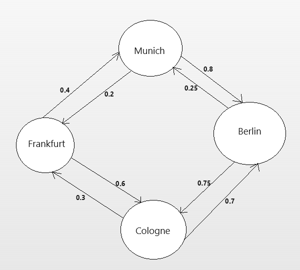
Fig 2: A fictitious Markov model of a transportation company and the routes randomly used by their clients.

Let us interpret the Markov Chain above. We can observe that 40% of the passengers who board in Frankfurt tend to disembark in Munich, while the other 60% tend to go to Cologne. Among the passengers in Cologne, 30% tend to return to Frankfurt, and 70% typically move on to Berlin. This model clearly highlights the most popular routes used by your customers.

Additionally, note that there are destinations with no direct connections. The absence of a connection indicates that, over the company's 70-year history, no customers have ever needed to travel directly between those two cities. Therefore, as the manager, you can confidently conclude that adding buses from Frankfurt to Berlin may not be as profitable compared to other popular routes, such as Frankfurt to Cologne.

The point being illustrated is that a transition matrix shows the different probabilities of transitioning from one state to another. According to Andrey Markov, the probability of you transitioning to any state only depends on your current state. It helps us understand how a system changes and which state it is most likely to transition into next. Before we can apply transition matrices to financial markets, we must first define all the possible states the market can be in.

Building Our Strategy: Defining Market States

One effective way to define market states is by using technical indicators. In the example below, we have applied a moving average to a symbol from our MetaTrader 5 Terminal. We can define the states as follows: "Whenever a candle closes above the moving average, the state is UP (1 in the diagram), and whenever a candle closes below the moving average, the state is DOWN (2 in the diagram)."

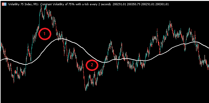
Fig 3: A schematic diagram showing the state of the market as either 1 or 2.

We can construct a Markov Chain to model how the market transitions from closing above the moving average to closing below it. In other words, a Markov Chain modeling the relationship between the moving average and the close price would answer questions such as, "If one candle closes above the moving average, what is the probability that the next candle will also close above the moving average?" If this probability exceeds 0.5, the market may be suitable for trend-following strategies. Otherwise, the market is more likely suitable for mean-reverting strategies.

Getting Started: Building Our First Transition Matrix

To get started, we start by importing our standard python libraries for communicating with our MetaTrader5 terminal and for data analysis.

#Import packages
import pandas as pd
import numpy as np
import MetaTrader5 as mt5
from   datetime import datetime
import pandas_ta as ta
import time

Then we have to define our login credentials and specify other global variables of interest such as the symbol we wish to trade, and the time frame we want to use. 

#Account login details
login = 123456789
password = "Enter Your Password"
server = "Enter Your Server"
symbol = "EURUSD"
#What timeframe are we working on?
timeframe = mt5.TIMEFRAME_M1
#This data frame will store the most recent price update
last_close = pd.DataFrame()
#We may not always enter at the price we want, how much deviation can we tolerate?
deviation = 100
#The size of our positions
volume = 0
#How many times the minimum volume should our positions be
lot_multiple = 1

Now, we can log in.

#Login
if(mt5.initialize(login=login,password=password,server=server)):
    print("Logged in successfully")
else:
    print("Failed to login")

Logged in successfully

Moving on, we now define our trading volume.

#Setup trading volume
symbols = mt5.symbols_get()
for index,symbol in enumerate(symbols):
    if symbol.name == "EURUSD":
        print(f"{symbol.name} has minimum volume: {symbol.volume_min}")
        volume = symbol.volume_min * lot_multiple

EURUSD has minimum volume: 0.01

We now need to specify how much data we need from our MetaTrader5 Terminal.

#Specify date range of data to be collected
date_start = datetime(2020,1,1)
date_end = datetime.now()

After fetching the data, we can now proceed to calculate our transition matrix to see how the EUR USD market evolves.

#Fetch market data
market_data = pd.DataFrame(mt5.copy_rates_range("EURUSD",timeframe,date_start,date_end))
market_data["time"] = pd.to_datetime(market_data["time"],unit='s')
#Add simple moving average technical indicator
market_data.ta.sma(length=20,append=True)
#Delete missing rows
market_data.dropna(inplace=True)
#Inspect the data frame
market_data

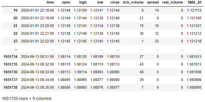
Fig 4: Our data frame in its current format.

We need to define how much space must be between the two candles of interest. In this example, we are interested in answering the question “If the current candle closes above the moving average, what is the probability the next candle will also close above the moving average?” If you are interested in the transition probabilities over greater time horizons, this is the parameter you should increase to meet your specific strategies needs.

#Define how far ahead we are looking
look_ahead = 1

Calculating a transition matrix is easy:

1. First, define all possible states (We defined 2 simple states, UP and DOWN).
2. Count how many candles fall into each respective state.
3. Calculate what proportion of all candles in the UP state were followed by another candle in the same state.
4. Calculate what proportion of all candles in the DOWN state were followed by another candle in the same state.

#Count the number of times price was above the moving average
up = market_data.loc[market_data["close"] > market_data["SMA_20"]].shape[0]

#Count the number of times price was below the moving average
down = market_data.loc[market_data["close"] < market_data["SMA_20"]].shape[0]

#Count the number of times price was above the moving average and remained above it
up_and_up = (market_data.loc[( (market_data["close"] > market_data["SMA_20"]) & (market_data["close"].shift(-look_ahead) > market_data["SMA_20"].shift(-look_ahead)) )].shape[0]) / up

#Count the number of times price was below the moving average and remained below it
down_and_down = (market_data.loc[( (market_data["close"] < market_data["SMA_20"]) & (market_data["close"].shift(-look_ahead) < market_data["SMA_20"].shift(-look_ahead)) )].shape[0]) / down

Then we combine the data into a data frame.

transition_matrix = pd.DataFrame({
    "UP":[up_and_up,(1-down_and_down)],
    "DOWN":[(1-up_and_up),down_and_down]
},index=['UP','DOWN'])

Let's view our transition matrix.

transition_matrix

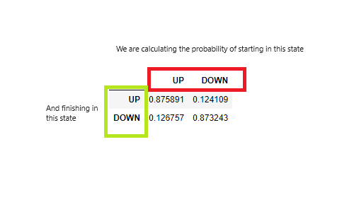
Fig 5: Our transition matrix.

Let us interpret the transition matrix together, our matrix is informing us that if the current candle closes above the moving average, there is an 88% chance the next candle will also close above the moving average and a 12% chance the next candle will close below the moving average. This is a good sign that moves in this particular market do not reverse themselves that often. Therefore, the market may be conformable to trend following strategies. 

Now that we have built our transition matrix, we can now build out the rest of our algorithm that will use this transition matrix to guide its decisions on whether it should buy or sell a particular security. 

We first define a function that will fetch the current price data from our terminal, and calculate our technical indicator values.

def get_prices():
    start = datetime(2024,6,1)
    end   = datetime.now()
    data  = pd.DataFrame(mt5.copy_rates_range("EURUSD",timeframe,start,end))
    #Add simple moving average technical indicator
    data.ta.sma(length=20,append=True)
    #Delete missing rows
    data.dropna(inplace=True)
    data['time'] = pd.to_datetime(data['time'],unit='s')
    data.set_index('time',inplace=True)
    return(data.iloc[-1,:])

Next, we will define a function to get the current state of the market.

def get_state(current_data):
    #Price is above the moving average, UP state
    if(current_data["close"]  > current_data["SMA_20"]):
        return(1)
    #Price is below the moving average, DOWN state
    elif(current_data["close"] < current_data["SMA_20"]):
        return(2)

Finally, we will define a function to select an action given the current state of the market and the transition probability.

def get_action(current_state):
    if(current_state == 1):
        if(transition_matrix.iloc[0,0] > transition_matrix.iloc[0,1]):
            print("The market is above the moving average and has strong trends, buy")
            print("Opening a BUY position")
            mt5.Buy("EURUSD",volume)
        elif(transition_matrix.iloc[0,0] < transition_matrix.iloc[0,1]):
            print("The market is above the moving average and has strong mean reverting moves, sell")
            print("Opening a sell position")
            mt5.Sell("EURUSD",volume)
    elif(current_state == 2):
        if(transition_matrix.iloc[1,0] > transition_matrix.iloc[1,1]):
            print("The market is below the moving average and has strong mean reverting moves, buy")
            print("Opening a BUY position")
            mt5.Buy("EURUSD",volume)
        elif(transition_matrix.iloc[1,0] < transition_matrix.iloc[1,1]):
            print("The market is below the moving average and has strong trends, sell")
            print("Opening a sell position")
            mt5.Sell("EURUSD",volume)

Now we can see our algorithm in action.

while True:
    #Get data on the current state of our terminal and our portfolio
    positions = mt5.positions_total()
    #If we have no open positions then we can open one
    if(positions == 0):
        get_action(get_state(get_prices()))
    #If we have finished all checks then we can wait for one day before checking our positions again
    time.sleep(60)

The market is below the moving average and has strong trends, sell.

Opening a sell position.

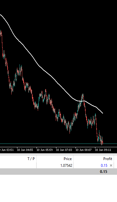
Fig 6: The trade selected by our trading algorithm.

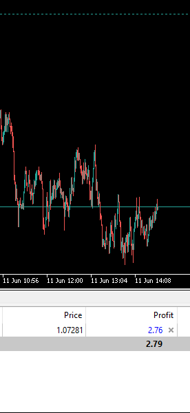
Fig 7: The trade selected by our trading algorithm the following day.

This is not all that can be said about transition matrices. However, it is a good introduction to the topic. Before we conclude our discussion, it is important we discuss which variables affect our transition matrix and how we can manipulate the transition matrix if need be.

The Symbol

The first variable that affects our transition matrix is obviously the symbol of choice, for example if we leave all other variables the same and simply select a new symbol, “Boom 1000 Index”, this what our transition matrix looks like now.

	UP	DOWN
UP	0.926	0.074
DOWN	0.043	0.957

As you can observe, when we selected the EURUSD as our symbol, the probability of seeing 2 consecutive candles above the moving average was 88% but now with this new symbol we have selected, "Boom 1000 Index" the probability of seeing 2  consecutive candles above the moving average has increased to 93%. Therefore, the symbol of choice has an undeniable effect on the transition matrix.

The Technical Indicator Parameters

Recall that we used technical indicators to help us easily define market states relative to the indicator. Therefore, changing the period of the moving average would greatly affect the transition matrix. To simply illustrate the point, we will go back to our initial conditions of modeling the EURUSD, but this time the only difference is that we will use a period of 2, whereas in our initial example we used a period of 20. All other variables are being held constant.

	UP	DOWN
UP	0.456	0.544
DOWN	0.547	0.453

Notice how the transition probabilities are now converging towards 50/50 chances of going in either direction. This implicitly tells us that as our moving average period gets larger, our transition probabilities grow further away from just 50/50 chances.

Gap Between The Candles

In our discussion, we were only concerned about the relationship between two consecutive candles. However, as we increase the gap between the candles under scrutiny, our transition matrix also changes. Again, we will go revert to the initial conditions we used to model the EURUSD however this time, we will increase the gap between the 2 candles to be 100. So all other variables will be the same, except for the gap between the 2 candles.

	UP	DOWN
UP	0.503	0.497
DOWN	0.507	0.493

Recommendations 

There is no absolute ‘right’ or ‘wrong’ way of designing your Markov Chain, however for your application to be consistent with our discussion it is imperative you follow the design pattern outlined below when building your Markov Chains:

transition_matrix = pd.DataFrame({
    "UP":["UP AND UP","UP AND DOWN"],
    "DOWN":["DOWN AND UP","DOWN AND DOWN"]
},index=['UP','DOWN'])

Our transition matrix is designed to quickly show us whether we should follow the trend or play against the trends.

Trend following strategies may work best when the main diagonal contains the largest probabilities, this means the market tends to pick up a trend, it tends to stay in the trend:

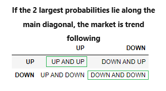
Fig 8: A trend following transition matrix.

Conversely, mean reverting strategies may work best when the off-diagonal contains the largest probabilities, this means the market tends to revert to equilibrium levels:

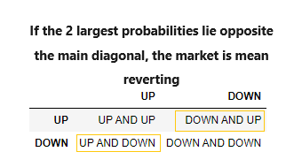
Fig 9: A mean reverting transition matrix.

Furthermore, if the largest probabilities are found in the bottom row, this means the market is bearish:

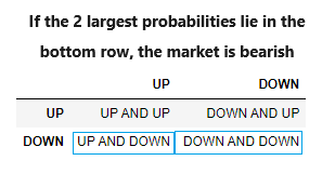
Fig 10: A bearish transition matrix.

Lastly, if the largest probabilities are found in the top row, this means the market is bullish:

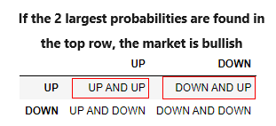
Fig 11: A bullish transition matrix.

MQL5 Implementation

We will now proceed to implement the strategy using MQL5 so that we can extensively test the strategy using real market data.

First, we load the libraries we need.

//+------------------------------------------------------------------+
//|                                          Transition Matrices.mq5 |
//|                                       Gamuchirai Zororo Ndawana. |
//|                                             https://www.mql5.com |
//+------------------------------------------------------------------+
#property copyright "Gamuchirai Zororo Ndawana."
#property link      "https://www.mql5.com"
#property version   "1.00"

//+------------------------------------------------------------------+
//|Overview                                                          |
//+------------------------------------------------------------------+
/*
This expert advisor will demonstrate how we can use transition matrices to build
self optimizing expert advisors. We will use the transition matrix to decide whether
we should employ trend following, or mean reverting trading strategies.

Gamuchirai Zororo Ndawana
Friday 19 July 2024, 10:09
Selebi Phikwe
Botswana
*/

//+------------------------------------------------------------------+
//| Libraries                                                        |
//+------------------------------------------------------------------+
#include <Trade/Trade.mqh>//Trade class
CTrade Trade;

Next, we define input parameters that can be edited by the end user.

//+------------------------------------------------------------------+
//| Inputs                                                            |
//+------------------------------------------------------------------+
input int fetch = 5; //How much historical data should we fetch?
input int look_ahead = 1; //Our forecast horizon

input int ma_period = 20; //The MA Period
input int rsi_period = 20; //The RSI Period
input int wpr_period = 20; //The Williams Percent Range Period

input int  lot_multiple = 20; //How big should the lot sizes be
input double sl_width = 0.4; //Stop loss size

Moving on, there are global variables we will need throughout our application.

//+------------------------------------------------------------------+
//|Global variables                                                  |
//+------------------------------------------------------------------+
double minimum_volume;//Smallest lot size
double ask_price;//Ask
double bid_price;//Bid
int ma_handler,rsi_handler,wpr_handler;//The handlers for our technical indicators
vector ma_readings(fetch);//MA indicator values
vector rsi_readings(fetch);//RSI indicator values
vector wpr_readings(fetch);//WPR indicator values
vector price_readings(fetch);//The vector we will use to store our historical price values
matrix transition_matrix = matrix::Zeros(2,2);//The matrix to store our observations on price's transition behavior
bool transition_matrix_initialized = false;//This flag will instruct the application to initialize the transition matrix
double up_and_up = 0;//These variables will keep count of the price transitions
double up_and_down = 0;
double down_and_up = 0;
double down_and_down = 0;
double total_count = (double) fetch - look_ahead;//This variable will store the total number of observations used to calculate the transition matrix
double trading_volume;//This is our desired trading size
vector market_behavior = vector::Zeros(4);//Transition matrix interpretations

We need to define the initialization function for our Expert Advisor, this function will ensure that our user passed valid inputs and set up our technical indicators.

//+------------------------------------------------------------------+
//| Initialization Function                                          |
//+------------------------------------------------------------------+
int OnInit()
  {
//--- Initialize the technical indicator
   ma_handler = iMA(_Symbol,PERIOD_CURRENT,ma_period,0,MODE_EMA,PRICE_CLOSE);
   rsi_handler = iRSI(_Symbol,PERIOD_CURRENT,rsi_period,PRICE_CLOSE);
   wpr_handler = iWPR(_Symbol,PERIOD_CURRENT,wpr_period);
   minimum_volume = SymbolInfoDouble(_Symbol,SYMBOL_VOLUME_MIN);
   trading_volume = minimum_volume * lot_multiple;
//--- Look ahead cannot be greater than fetch
   if(look_ahead > fetch)
     {
      Comment("We cannot forecast further into the future than thr to total amount of  data fetched.\nEither fetch more data or forecast nearer to the present.");
      return(INIT_FAILED);
     }
//--- End of initialization
   return(INIT_SUCCEEDED);
  }

Our program also needs a procedure to follow whenever it is de-initialized.

//+------------------------------------------------------------------+
//| Expert de-initialization function                                |
//+------------------------------------------------------------------+
void OnDeinit(const int reason)
  {
//--- Remove technical indicators
   IndicatorRelease(rsi_handler);
   IndicatorRelease(wpr_handler);
   IndicatorRelease(ma_handler);
//--- Remove Expert Advisor
   ExpertRemove();
  }

We'll also make a function to update our technical indicators and fetch current market prices.

//+------------------------------------------------------------------+
//|This function will update our technical indicator values          |
//+------------------------------------------------------------------+
void update_technical_indicators(void)
  {
//--- Update bid and ask price
   ask_price = SymbolInfoDouble(_Symbol,SYMBOL_ASK);
   bid_price = SymbolInfoDouble(_Symbol,SYMBOL_BID);
//--- Update each indicator value, we only need the most recent reading
   rsi_readings.CopyIndicatorBuffer(rsi_handler,0,0,1);
   wpr_readings.CopyIndicatorBuffer(wpr_handler,0,0,1);
   ma_readings.CopyIndicatorBuffer(ma_handler,0,0,1);
  }

Remember that our interpretations of the technical indicator readings will always depend on the behavior of the market as measured by the transition matrix.

//+------------------------------------------------------------------+
//|This function will find an entry opportunity based on our signals |                                                                  |
//+------------------------------------------------------------------+
void find_entry(void)
  {
//--- Store the index of our largest entry
   ulong max_arg = market_behavior.ArgMax();

//--- First we have to know the behavior of the market before we decide to buy or sell
   if(max_arg == 0)
     {
      //--- This means that the market is bullish and we should probably only take buy oppurtunities
      Comment("The observed transition matrix can only be generated by a bullish market");
      bullish_sentiment(0);
     }
   else
      if(max_arg == 1)
        {
         //--- This means that the market is bearish and we should probably only take sell oppurtunities
         Comment("The observed transition matrix can only be generated by a bearish market");
         bearish_sentiment(0);
        }
      else
         if(max_arg == 2)
           {
            //--- This means that the market trends and we should probably join either side of the trend
            Comment("The observed transition matrix can only be generated by a trending market");
            bearish_sentiment(0);
            bullish_sentiment(0);
           }
         else
            if(max_arg == 3)
              {
               //--- This means that the market is mean reverting and we should probably play against the trends on either side
               Comment("The observed transition matrix can only be generated by a mean reverting market");
               bearish_sentiment(-1);
               bullish_sentiment(-1);
              }
  }

We need a function to execute our long orders.

//+----------------------------------------------------------------+
//|This function will look for oppurtunities to buy                |
//+----------------------------------------------------------------+
void bullish_sentiment(int f_flag)
  {
//--- This function analyses the market for bullish sentiment using our technical indicator
//--- It has only 1 parameter, a flag denoting whether we should interpret the indicators in a trend following fashion
//--- or a mean reverting fashion. For example 0 means interpret the indicators in a trend following fashion.
//--- Therefore if we call the function and pass 0, RSI readings above 50 will trigger buy orders.
//--- However if -1 was passed then RSI readings below 50 will trigger buy orders.
//--- First make sure we have no open positions
   if(PositionsTotal() > 0)
     {
      return;
     }

//--- Interpret the flag
   if(f_flag == 0)
     {
      //--- The flag is telling us to follow the trend
      if((rsi_readings[0] > 50) && (wpr_readings[0] > -50))
        {
         Trade.Buy(trading_volume,_Symbol,ask_price,(ask_price - sl_width),(ask_price + sl_width),"Transition Matrix Order");
        }
     }
   else
      if(f_flag == -1)
        {
         //--- The flag is telling us to bet against the trend
         if((rsi_readings[0] < 50) && (wpr_readings[0] < -50))
           {
            Trade.Buy(trading_volume,_Symbol,ask_price,(ask_price - sl_width),(ask_price + sl_width),"Transition Matrix Order");
           }
        }

  }

This function will execute our short orders for us. Recall that if our market is mean reverting, then we will interpret the indicators in the "opposite" way.

//+-------------------------------------------------------------+
//|This function will help us find oppurtunities to sell        |
//+-------------------------------------------------------------+
void bearish_sentiment(int f_flag)
  {
//--- This function analysises the market for bearish sentiment using our technical indicator
//--- It has only 1 parameter, a flag denoting whether we should interpret the indicators in a trend following fashion
//--- or a mean reverting fashion. For example 0 means interpret the indicators in a trend following fashion.
//--- Therefore if we call the function and pass 0, RSI readings below 50 will trigger sell orders.
//--- However if -1 was passed then RSI readings above 50 will trigger sell orders.
//--- First make sure we have no open positions
   if(PositionsTotal() > 0)
     {
      return;
     }
//--- Interpret the flag
   if(f_flag == 0)
     {
      //--- Now we know how to interpret our technical indicators
      if((rsi_readings[0] < 50) && (wpr_readings[0] < -50))
        {
         Trade.Sell(trading_volume,_Symbol,bid_price,(bid_price + sl_width),(bid_price - sl_width),"Transition Matrix Order");
        }
     }
   else
      if(f_flag == -1)
        {
         //--- Now we know how to interpret our technical indicators
         if((rsi_readings[0] > 50) && (wpr_readings[0] > -50))
           {
            Trade.Sell(trading_volume,_Symbol,bid_price,(bid_price + sl_width),(bid_price - sl_width),"Transition Matrix Order");
           }
        }
  }

Let us also define a function that will ensure our transition matrix is prepared and calculated according to the procedure we outlined above.

//+---------------------------------------------------------------+
//|This function will initialize our transition matrix            |
//+---------------------------------------------------------------+
void initialize_transition_matrix(void)
  {
//--- We need to update our historical price readings and our MA readings
   ma_readings.CopyIndicatorBuffer(ma_handler,0,1,fetch);
   price_readings.CopyRates(_Symbol,PERIOD_CURRENT,COPY_RATES_CLOSE,1,fetch);

//--- Now let us update our transition matrix
   for(int i = 0; i < fetch - look_ahead; i++)
     {
      //--- Did price go from being above the MA but end up beneath the MA?
      if((price_readings[i] > ma_readings[i]) && (price_readings[i + look_ahead] < ma_readings[i + look_ahead]))
        {
         up_and_down += 1;
        }
      //--- Did price go from being above the MA and remain above it?
      else
         if((price_readings[i] > ma_readings[i]) && (price_readings[i + look_ahead] > ma_readings[i + look_ahead]))
           {
            up_and_up += 1;
           }

         //--- Did price go from being below the MA but end up above it?
         else
            if((price_readings[i] < ma_readings[i]) && (price_readings[i + look_ahead] > ma_readings[i + look_ahead]))
              {
               down_and_up += 1;
              }

            //--- Did price go from being below the MA and remain below it?
            else
               if((price_readings[i] < ma_readings[i]) && (price_readings[i + look_ahead] < ma_readings[i + look_ahead]))
                 {
                  down_and_down += 1;
                 }
     }

//--- Let us see our counts so far
   Print("Up and up: ",up_and_up,"\nUp and down: ",up_and_down,"\nDown and up: ",down_and_up,"\nDown and down: ",down_and_down);
   double sum_of_counts = up_and_up + up_and_down + down_and_up + down_and_down;
   Print("Sum of counts: ",(sum_of_counts),"\nObservations made: ",total_count,"\nDifference:[the difference should always be 0] ",(total_count - sum_of_counts));
//--- Now we will calculate the transition matrix
//--- The matrix position (0,0) stores the probaility that after making a move up, the market will continue rising
//--- The matrix position (0,1) stores the probability that after making a move down, price will reverse and start rising
//--- The matrix position (1,0) stores the probability that after making a move up, price will reverse and start falling
//--- The matrix position (1,1) stores the probabilty that after making a move down, price will continue falling
   transition_matrix[0][0] = up_and_up / (up_and_up + up_and_down);
   transition_matrix[0][1] = down_and_up / (up_and_up + up_and_down);
   transition_matrix[1][0] = up_and_down / (down_and_up + down_and_down);
   transition_matrix[1][1] = down_and_down / (down_and_up + down_and_down);
//--- Show the transition matrix
   Print("Our transition Matrix");
   Print(transition_matrix);
//--- Now we need to make sense of the transition matrix
   analyse_transition_matrix();
//--- Now we need to update the flag
   transition_matrix_initialized = true;
  }

We also need a helper function to interpret our transition matrix.

//+-------------------------------------------------------------+
//|This function will analyse our transition matrix             |
//+-------------------------------------------------------------+
void analyse_transition_matrix(void)
  {
//--- Check if the market is bullish
   if((transition_matrix[0][0] > transition_matrix[1][0])&&(transition_matrix[0][1] > transition_matrix[1][1]))
     {
      market_behavior[0] = 1;
     }
//--- Check if the market is bearish
   else
      if((transition_matrix[0][1] > transition_matrix[1][0])&&(transition_matrix[1][1] > transition_matrix[1][0]))
        {
         market_behavior[1] = 1;
        }
      //--- Check if the market trends
      else
         if(transition_matrix.Trace() > 1)
           {
            market_behavior[2] = 1;
           }
         //--- Check if the market is mean reverting
         else
            if(transition_matrix.Trace() < 1)
              {
               market_behavior[3] = 1;
              }
  }
//+------------------------------------------------------------------+

Our OnTick handler will ensure that all the functions we outlined above will be called at the appropriate time.

//+------------------------------------------------------------------+
//| Expert tick function                                             |
//+------------------------------------------------------------------+
void OnTick()
  {
//--- First we must check if our transition matrix has been initialized
   if(!transition_matrix_initialized)
     {
      initialize_transition_matrix();
     }
//--- Otherwise our transition matrix has been initialized
   else
     {
      //--- Update technical indicator values
      update_technical_indicators();
      //--- If we have no open positions we will use our tranistion matrix to help us interpret our technical indicators
      if(PositionsTotal() == 0)
        {
         find_entry();
        }
     }
  }
//+------------------------------------------------------------------+

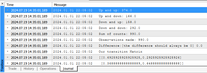
Fig 12: Our Transition Matrix calculated in MQL5.

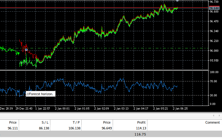
Fig 13: Our Expert Advisor trading the AUDJPY pair.

Conclusion

This article explores the application of Markov Chains in algorithmic trading to adapt to changing market conditions. Beginning with an introduction to the concept of Markov Chains, we illustrate their usefulness in modeling random processes akin to market dynamics. By defining market states using technical indicators, such as moving averages, we demonstrate how to construct a Markov Chain to analyze market transitions. This approach allows us to determine the probability of future market movements, helping us decide whether to employ trend-following or mean-reverting strategies. Through this method, we aim to create intelligent trading algorithms with enhanced decision-making capabilities, ultimately improving trading performance in dynamic markets.