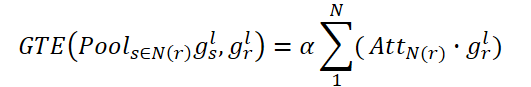
Neural networks made easy (Part 80): Graph Transformer Generative Adversarial Model (GTGAN)

Introduction
The initial state of the environment is most often analyzed using models that utilize convolutional layers or various attention mechanisms. However, convolutional architectures lack understanding of long-term dependencies in the original data due to inherent inductive biases. Architectures based on attention mechanisms allow the encoding of long-term or global relationships and the learning of highly expressive feature representations. On the other hand, graph convolution models make good use of local and neighboring vertex correlations based on the graph topology. Therefore, it makes sense to combine graph convolution networks and Transformers to model local and global interactions in an attempt to implement the search for optimal trading strategies.
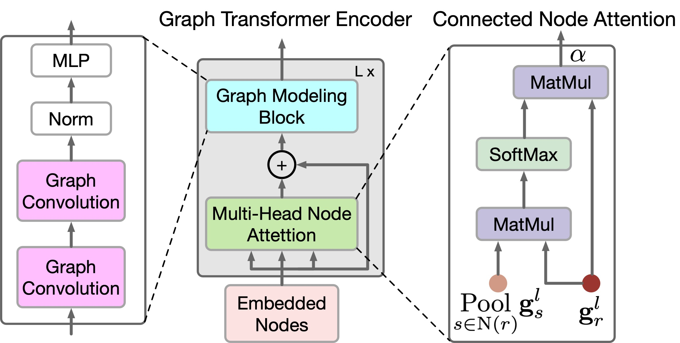
The recently published paper "Graph Transformer GANs with Graph Masked Modeling for Architectural Layout Generation" introduces the algorithm for the graph transformer generative adversarial model (GTGAN), which succinctly combines both of these approaches. The authors of the GTGAN algorithm address the problem of creating a realistic architectural design of a house from an input graph. The generator model they presented consists of three components: a message passing convolutional neural network (Conv-MPN), Graph Transformer encoder (GTE) and generation head.
Qualitative and quantitative experiments on three complex graphically constrained architectural layout generations with three datasets that were presented in the paper demonstrate that the proposed method can generate results superior to previously presented algorithms.
1. GTGAN algorithm
To describe the method, let's use the creation of a house layout as an example. Generator G receives the noise vector for each room and the bubble chart as input. It then generates a house layout in which each room is represented as an axis-aligned rectangle. The authors of the method represent each bubble chart as a graph, where each node represents a room of a certain type, and each edge represents the spatial adjacency of rooms. Specifically, they generate a rectangle for each room. Two rooms with a graph edge should be spatially adjacent, while two rooms without a graph edge should be spatially dis-adjacent.
Given a bubble diagram, they first generate a node for each room and initialize it with a 128-dimensional noise vector sampled from a normal distribution. Then they combine the noise vector with a 10-dimensional one-hot room type vector (tr). Therefore, they can obtain a 138 dimensional vector gr to represent the original bubble diagram.
![]()
Note that in this case, the graph nodes are used as the input data of the proposed transformer.
Convolutional message passing block Conv-MPN represents a 3D tensor in the output design space. They apply a general line layer to expand gr into a feature volume gr,l=1 of size 16×8×8, where l=1 is the object extracted from the first Conv-MPN layer. It will be upsampled twice using a transposed convolution to become an object gr,l=3 of size 16x32x32.
The Conv-MPN layer updates the feature graph by passing convolutional messages. Specifically, they update gr,l=1 over the following steps:
- They use one GTE to capture long-term correlations across rooms that are connected in the input graph;
- The use another GTE to capture long-term dependencies across non-connected rooms in the input graph;
- They combine functions across connected rooms in the input graph;
- The combine functions across unrelated rooms;
- We apply a convolutional block (CNN) on the combined feature.
This process can be formulated as follows:
![]()
where N(r) denote sets of rooms that are connected and not-connected, respectively; "+" and ";" denote pixel-wise addition and channel-wise concatenation, respectively.
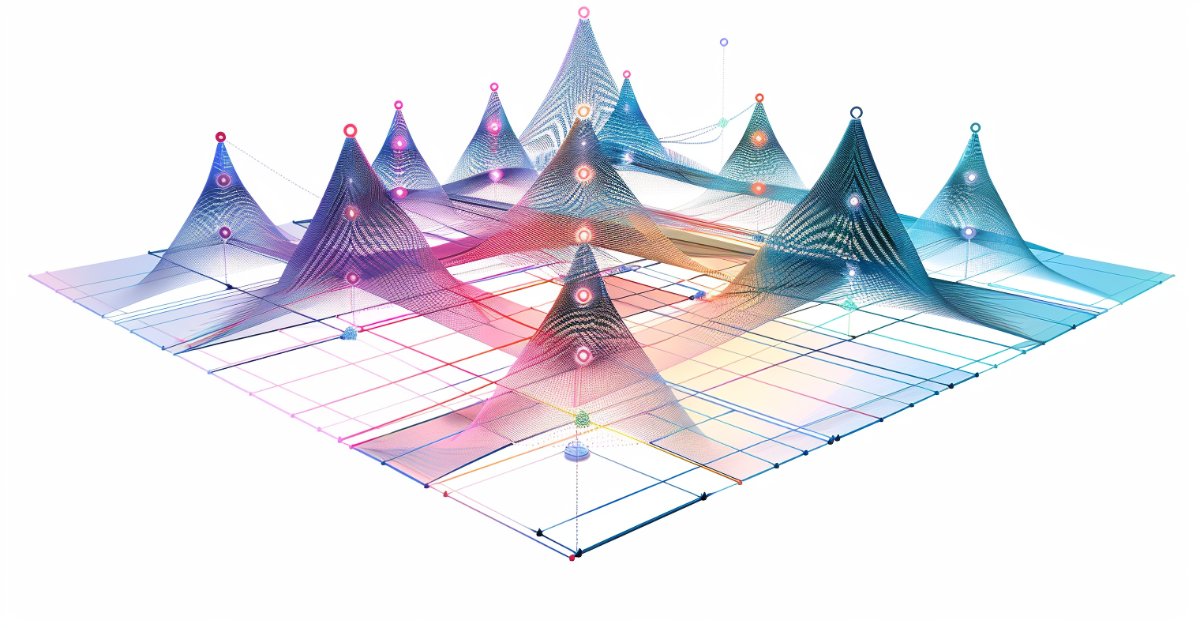
To reflect local and global relationships between graph nodes, the authors of the method propose a new GTE encoder. GTE combines Self-Attention of the Transformer and Graph Convolution models to capture global and local correlations, respectively. Please note that GTGAN does not use positional embeddings since the goal of the task is to indicate the positions of the nodes in the generated house layout.
GTGAN expands multi-head Self-Attention into the multi-head node attention which aims to capture global correlations between connected rooms/nodes and global dependencies between unconnected rooms/nodes. For this purpose, the authors of the method propose two new graph node attention modules, namely: connected node attention (CNA) and non-connected node attention (NNA). Both modules have the same network architecture.
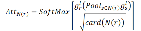
The goal of CNA is to model global correlations across connected rooms. AttN(r) measures the influence of a node on other connected nodes. Then they perform matrix multiplication gr,l by the transposed AttN(r). After that they multiply the result by the scaling parameter ɑ.
Where ɑ is a learnable parameter.
Each connected node in N(r) represents the weighted sum of all connected nodes. Thus, CNA obtains a global view of the spatial graph structure and can selectively adjust rooms according to the connected attention map, improving the house layout representation and high-level semantic consistency.
Similarly, NNA aims to capture global relationships in non-connected rooms. It uses its learnable parameter ß.
Finally, they perform element-wise sum of gr,l so that the updated node feature can capture both connected and non-connected spatial relations.
![]()
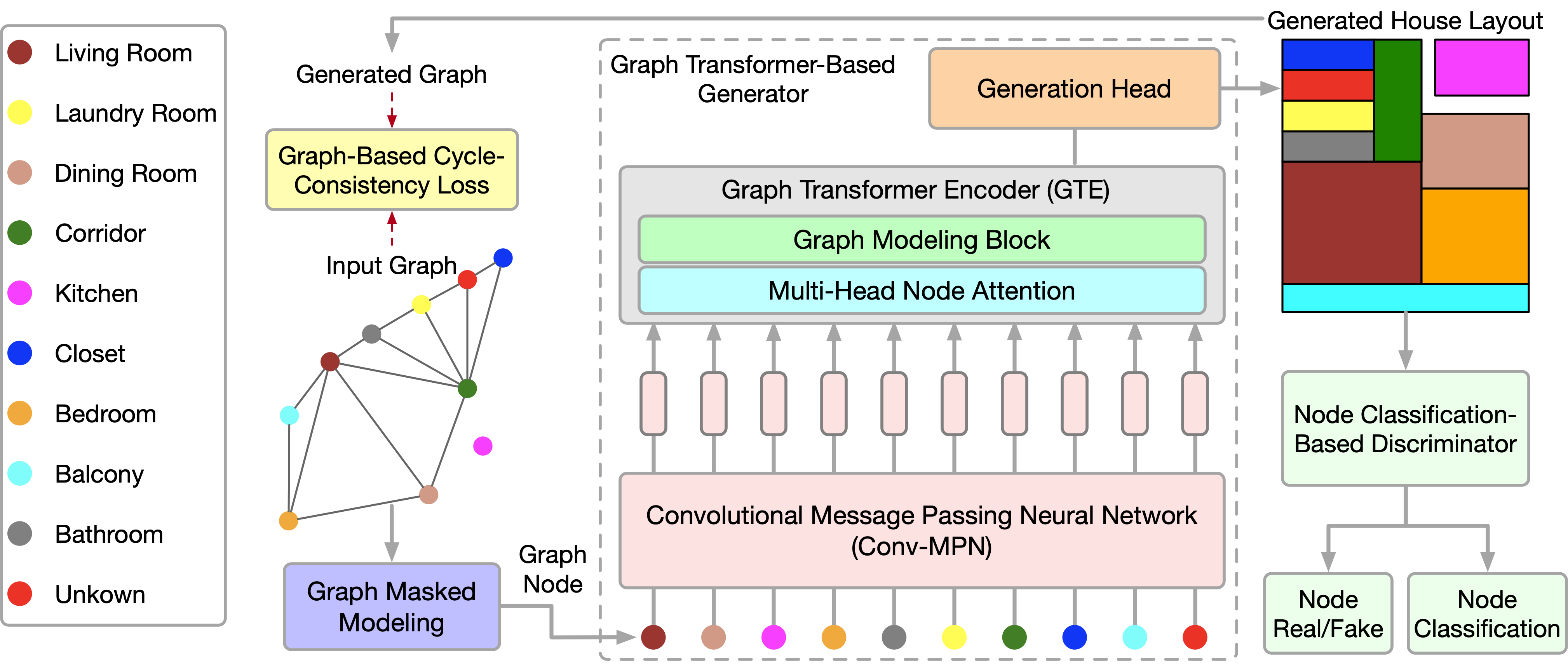
While CNA and NNA are useful for extracting long-term and global dependencies, they are less effective at capturing fine-grained local information in complex home data structures. To fix this limitation, the authors of the method propose a new graph modeling block.
Specifically, given the features gr,l, generated in the equation above, they further improve local correlations using convolutional graph networks.
![]()
Where A denotes the adjacency matrix of the graph, G.C.(•) represents the convolution of the graph, and P denotes the learnable parameters. σ is the linear Gaussian error unit (GeLU).
Providing information about the relationships of nodes in the global graph helps create more accurate house layouts. To differentiate this process, the authors of the method propose a new loss function based on an adjacency matrix that corresponds to the spatial relationships between the ground truth and the generated graphs. Precisely, the graphs capture the adjacency relationships between each node in different rooms, and then ensure the correspondence between the ground truth and the generated graphs through the proposed loop consistency loss function. This loss function aims to accurately maintain mutual relationships between nodes. On the one hand, non-overlapping parts must be predicted as non-overlapping. On the other hand, neighboring nodes must be predicted as neighbors and correspond to proximity coefficients.
The authors' visualization of GTGAN is presented below.
2. Implementation using MQL5
After considering the theoretical aspects of the GTGAN method, we move on to the practical part of our article, in which we implement the proposed approaches using MQL5.
However, please pay attention to the difference between the problems solved by the authors of the method and those solved by us. Our goal is not to generate a price movement chart. Our goal is to find the optimal behavior strategy for the Agent. At the output of the model, we want to obtain the optimal action of the Agent in a particular state of the environment. At first glance, our tasks are radically different.
But if you take a closer look at the GTGAN methodology, then you can see that the method authors mainly focus on the Encoder (GTE). They pay much attention to both the encoder architecture and its training.
The authors of the method propose preliminary training of the Encoder with random masking of both nodes and connections. They propose to mask up to 40% of the original data, leaving each node and edge with potential gaps in neighboring connections. To recover missing data, each node and edge embedding must consume and interpret its local context. That is, each investment must understand specific details of its immediate environment. The proposed approach of high-ratio random masking and subsequent reconstruction overcomes the limitations imposed by the size and shape of the subgraphs used for prediction. As a result, node and edge embeddings are encouraged to understand local contextual details.
In addition, when nodes or edges with high coefficients are removed, the remaining nodes and edges can be considered as a set of subgraphs whose task is to predict the entire graph. This represents a more complex per-graph prediction task compared to other self-pretraining tasks, which typically capture global graph details using smaller graphs or context as prediction targets. The proposed "intensive" pre-training task of masking and graph reconstruction provides a broader perspective for learning superior node-edge embeddings capable of capturing complex details both at the level of individual nodes/edges and at the level of the entire graph.
The encoder in the proposed system acts as a bridge, transforming the original attributes of visible, unmasked nodes and edges into their corresponding embeddings in latent feature spaces. This process includes the node and edge aspects of the encoder, which include the proposed graph modeling block and multi-head node attention mechanism. These functions are designed in the spirit of the Transformer architecture, a technique known for its ability to efficiently model sequential data. This block helps create robust representations that encapsulate the holistic dynamics of relationships within a graph.
Consequently, we can use the proposed Encoder to study local and global dependencies in the source data. We will implement the proposed Encoder algorithm in a new class entitled CNeuronGTE.
2.1 GTE Encoder Class
The GTE encoder class CNeuronGTE will inherit form our neural layer base class CNeuronBaseOCL. The structure of the proposed Encoder is significantly different from the previously considered Transformer options. Therefore, despite the large number of previously created neural layers that use attention mechanisms, we decided to refuse to inherit one of them. Although in the process of work we will use previously created developments.
The structure of the new class is shown below.
class CNeuronGTE : public CNeuronBaseOCL
  {
protected:
   uint              iHeads;                                      ///< Number of heads
   uint              iWindow;                                     ///< Input window size
   uint              iUnits;                                      ///< Number of units
   uint              iWindowKey;                                  ///< Size of Key/Query window
   //---
   CNeuronConvOCL    cQKV;
   CNeuronSoftMaxOCL cSoftMax;
   int               ScoreIndex;
   CNeuronBaseOCL    cMHAttentionOut;
   CNeuronConvOCL    cW0;
   CNeuronBaseOCL    cAttentionOut;
   CNeuronCGConvOCL  cGraphConv[2];
   CNeuronConvOCL    cFF[2];
   //---
   virtual bool      feedForward(CNeuronBaseOCL *NeuronOCL);
   virtual bool      AttentionOut(void);
   //---
   virtual bool      updateInputWeights(CNeuronBaseOCL *NeuronOCL);
   virtual bool      AttentionInsideGradients(void);

public:
                     CNeuronGTE(void) {};
                    ~CNeuronGTE(void) {};
   //---
   virtual bool      Init(uint numOutputs, uint myIndex, COpenCLMy *open_cl,
                          uint window, uint window_key, uint heads,
                          uint units_count,
                          ENUM_OPTIMIZATION optimization_type,
                          uint batch);
   virtual bool      calcInputGradients(CNeuronBaseOCL *prevLayer);
   //---
   virtual int       Type(void)   const   {  return defNeuronGTE;   }
   //--- methods for working with files
   virtual bool      Save(int const file_handle);
   virtual bool      Load(int const file_handle);
   virtual CLayerDescription* GetLayerInfo(void);
   virtual void      SetOpenCL(COpenCLMy *obj);
   virtual void      TrainMode(bool flag);                ///< Set Training Mode Flag
  };
You can see here already familiar local variables:
- iHeads;
- iWindow;
- iUnits;
- iWindowKey.
Their functional purpose remains the same. We will get acquainted with the purpose of the internal layers while implementing the methods.
We declared all internal objects static, which allows us to leave the constructor and destructor of the class empty. Please note that in the class constructor, we do not even specify the value of local variables.
As always, complete initialization of the class is performed in the Init method. In the parameters of this method we receive all the necessary information to create the correct class architecture. In the body of the method, we call the relevant method of the parent class, which implements the minimum necessary control of the received initial parameters and initialization of inherited objects.
bool CNeuronGTE::Init(uint numOutputs, uint myIndex, COpenCLMy *open_cl,
                      uint window, uint window_key, uint heads,
                      uint units_count, ENUM_OPTIMIZATION optimization_type,
                      uint batch)
  {
   if(!CNeuronBaseOCL::Init(numOutputs, myIndex, open_cl, window * units_count, optimization_type, batch))
      return false;
After the successful execution of the parent class method, we save the received data into local variables.
   iWindow = fmax(window, 1);
   iWindowKey = fmax(window_key, 1);
   iUnits = fmax(units_count, 1);
   iHeads = fmax(heads, 1);
   activation = None;
Then initialize the added objects. First, we initialize the inner convolutional layer cQKV. In this layer, we plan to generate a representation of all 3 entities (Query, Key and Value) in parallel threads. The size of the source data window and its step is equal to the size of the description of one sequence element. The number of convolution filters is equal to the product of the size of the description vector of one entity of one element of the sequence multiplied by the number of attention heads and by 3 (the number of entities). The number of elements is equal to the size of the analyzed sequence.
   if(!cQKV.Init(0, 0, OpenCL, iWindow, iWindow, iWindowKey * 3 * iHeads, iUnits, optimization, iBatch))
      return false;
To increase the stability of the block, we normalize the generated entities using a SoftMax layer.
   if(!cSoftMax.Init(0, 1, OpenCL, iWindowKey * 3 * iHeads * iUnits, optimization, iBatch))
      return false;
   cSoftMax.SetHeads(3 * iHeads * iUnits);
The next step is to create a dependency coefficient buffer in the OpenCL context. Its size is 2 times larger than usual — this is needed to separately record the coefficients for connected and non-connected vertices.
   ScoreIndex = OpenCL.AddBuffer(sizeof(float) * iUnits * iUnits * 2 * iHeads, CL_MEM_READ_WRITE);
   if(ScoreIndex == INVALID_HANDLE)
      return false;
We will save the results of multi-head attention in the local layer cMHAttentionOut.
   if(!cMHAttentionOut.Init(0, 2, OpenCL, iWindowKey * 2 * iHeads * iUnits, optimization, iBatch))
      return false;
Please note that the size of the layer of multi-head attention results is also 2 times larger than the similar layer of the Transformer implementations considered earlier. This is also done to enable the writing of data from both connected and non-connected vertices.
In addition, with this approach, there is no need to implement a separate functionality for training the scaling parameters ɑ and ß. Instead, we will use the functionality of the W0 layer. In this case, it will combine attention heads, as well as the influence of connected and non-connected vertices.
   if(!cW0.Init(0, 3, OpenCL, 2 * iWindowKey * iHeads, 2 * iWindowKey* iHeads, iWindow, iUnits,
                                                                             optimization, iBatch))
      return false;
After the attention block, we need to add the results with the original data and normalize the results. The resulting values are written to the cAttentionOut layer.
   if(!cAttentionOut.Init(0, 4, OpenCL, iWindow * iUnits, optimization, iBatch))
      return false;
Next come 2 blocks of 2 layers each. These include a block of graph convolution and FeedForward. We initialize the objects of the specified blocks in a loop.
   for(int i = 0; i < 2; i++)
     {
      if(!cGraphConv[i].Init(0, 5 + i, OpenCL, iWindow, iUnits, optimization, iBatch))
         return false;
      if(!cFF[i].Init(0, 7 + i, OpenCL, (i == 0 ? iWindow : 4 * iWindow),
                      (i == 0 ? iWindow : 4 * iWindow),
                      (i == 1 ? iWindow : 4 * iWindow),
                      iUnits, optimization, iBatch))
         return false;
     }
Finally, let's replace the error gradient buffer.
   if(cFF[1].getGradient() != Gradient)
     {
      if(!!Gradient)
         delete Gradient;
      Gradient = cFF[1].getGradient();
     }
//---
   return true;
  }
This finishes the method.
After initializing the class, we proceed to organizing the algorithm for the feed-forward pass of the class. Here we begin with our OpenCL program, in which we have to create a new kernel GTEFeedForward. Within this kernel, we will analyze the dependencies of both connected and non-connected nodes. In the methodology of the GTGAN method, in the GTEFeedForward kernel body, we implement the functionality of CNA and NNA.
But, before moving on to implementation, let's determine which nodes should be considered connected and which non-connected. The first thing you need to know is that the nodes in our implementation are descriptions of the parameters of one bar. We are dealing with time series analysis. Therefore, we can only have 2 adjacent bars directly connected. Therefore, for the bar Xt, only bars Xt-1 and Xt+1 are connected. Bars Xt-1 and Xt+1 are not connected since there is bar Xt between them.
Now we can move on to the implementation. In the parameters, the kernel receives pointers to the data exchange buffers.
__kernel void GTEFeedForward(__global float *qkv,
                             __global float *score,
                             __global float *out,
                             int dimension)
  {
   const size_t cur_q = get_global_id(0);
   const size_t units_q = get_global_size(0);
   const size_t cur_k = get_local_id(1);
   const size_t units_k = get_local_size(1);
   const size_t h = get_global_id(2);
   const size_t heads = get_global_size(2);
In the kernel body, we identify a thread in the task space. In this case, we are dealing with a 3-dimensional space of tasks, one of which is combined into a local group.
The next step is to determine the mixtures in the data buffers.
   int shift_q = dimension * (cur_q + h * units_q);
   int shift_k = (cur_k + h * units_k + heads * units_q);
   int shift_v = dimension * (h * units_k + heads * (units_q + units_k));
   int shift_score_con = units_k * (cur_q * 2 * heads + h) + cur_k;
   int shift_score_notcon = units_k * (cur_q * 2 * heads + heads + h) + cur_k;
   int shift_out_con = dimension * (cur_q + h * units_q);
   int shift_out_notcon = dimension * (cur_q + units_q * (h + heads));
Here we will declare a 2-dimensional local array. The second dimension has 2 elements for connected and non-connected nodes.
   const uint ls_score = min((uint)units_k, (uint)LOCAL_ARRAY_SIZE);
   __local float local_score[LOCAL_ARRAY_SIZE][2];
The next step is to determine the dependence coefficients. First we multiply the corresponding Query and Key tensors. Divide it by the root of the dimension and take the exponential value.
//--- Score
   float scr = 0;
   for(int d = 0; d < dimension; d ++)
      scr += qkv[shift_q + d] * qkv[shift_k + d];
   scr = exp(min(scr / sqrt((float)dimension), 30.0f));
Then we determine whether the analyzed sequence elements are connected and save the result to the required buffer element.
   if(cur_q == cur_k)
     {
      score[shift_score_con] = scr;
      score[shift_score_notcon] = scr;
      if(cur_k < ls_score)
        {
         local_score[cur_k][0] = scr;
         local_score[cur_k][1] = scr;
        }
     }
   else
     {
      if(abs(cur_q - cur_k) == 1)
        {
         score[shift_score_con] = scr;
         score[shift_score_notcon] = 0;
         if(cur_k < ls_score)
           {
            local_score[cur_k][0] = scr;
            local_score[cur_k][1] = 0;
           }
        }
      else
        {
         score[shift_score_con] = 0;
         score[shift_score_notcon] = scr;
         if(cur_k < ls_score)
           {
            local_score[cur_k][0] = 0;
            local_score[cur_k][1] = scr;
           }
        }
     }
   barrier(CLK_LOCAL_MEM_FENCE);
Now we can find the sum of the coefficients for each of the elements of the sequence.
   for(int k = ls_score; k < units_k; k += ls_score)
     {
      if((cur_k + k) < units_k)
        {
         local_score[cur_k][0] += score[shift_score_con + k];
         local_score[cur_k][1] += score[shift_score_notcon + k];
        }
     }
   barrier(CLK_LOCAL_MEM_FENCE);
//---
   int count = ls_score;
   do
     {
      count = (count + 1) / 2;
      if(cur_k < count)
        {
         if((cur_k + count) < units_k)
           {
            local_score[cur_k][0] += local_score[cur_k + count][0];
            local_score[cur_k][1] += local_score[cur_k + count][1];
            local_score[cur_k + count][0] = 0;
            local_score[cur_k + count][1] = 0;
           }
        }
      barrier(CLK_LOCAL_MEM_FENCE);
     }
   while(count > 1);
   barrier(CLK_LOCAL_MEM_FENCE);
Then we bring the sum of the dependence coefficients to 1 for each element of the sequence. To do this, simply divide the value of each element by the corresponding sum.
   score[shift_score_con] /= local_score[0][0];
   score[shift_score_notcon] /= local_score[0][1];
   barrier(CLK_LOCAL_MEM_FENCE);
Once the dependence coefficients are found, we can determine the effects of connected and non-connected nodes.
   shift_score_con -= cur_k;
   shift_score_notcon -= cur_k;
   for(int d = 0; d < dimension; d += ls_score)
     {
      if((cur_k + d) < dimension)
        {
         float sum_con = 0;
         float sum_notcon = 0;
         for(int v = 0; v < units_k; v++)
           {
            sum_con += qkv[shift_v + v * dimension + cur_k + d] * score[shift_score_con + v];
            sum_notcon += qkv[shift_v + v * dimension + cur_k + d] * score[shift_score_notcon + v];
           }
         out[shift_out_con + cur_k + d] = sum_con;
         out[shift_out_notcon + cur_k + d] = sum_notcon;
        }
     }
  }
After successfully completing all iterations, we complete the kernel operation and return to working on the main program. Here we first create the AttentionOut method to call the kernel created above. This is a method that will be called from another method of the same class. It works only with internal objects and does not contain parameters.
In the body of the method, we first check the relevance of the pointer to the class object for working with the OpenCL context.
bool CNeuronGTE::AttentionOut(void)
  {
   if(!OpenCL)
      return false;
Then we determine the task space and the size of the working groups. In this case, we use a 3-dimensional task space with 1-dimensional grouping into work groups.
   uint global_work_offset[3] = {0};
   uint global_work_size[3] = {iUnits/*Q units*/, iUnits/*K units*/, iHeads};
   uint local_work_size[3] = {1, iUnits, 1};
Then we pass the necessary parameters to the kernel.
   ResetLastError();
   if(!OpenCL.SetArgumentBuffer(def_k_GTEFeedForward, def_k_gteff_qkv, cQKV.getOutputIndex()))
     {
      printf("Error of set parameter kernel %s: %d; line %d", __FUNCTION__, GetLastError(), __LINE__);
      return false;
     }
   if(!OpenCL.SetArgumentBuffer(def_k_GTEFeedForward, def_k_gteff_score, ScoreIndex))
     {
      printf("Error of set parameter kernel %s: %d; line %d", __FUNCTION__, GetLastError(), __LINE__);
      return false;
     }
   if(!OpenCL.SetArgumentBuffer(def_k_GTEFeedForward, def_k_gteff_out, cAttentionOut.getOutputIndex()))
     {
      printf("Error of set parameter kernel %s: %d; line %d", __FUNCTION__, GetLastError(), __LINE__);
      return false;
     }
   if(!OpenCL.SetArgument(def_k_GTEFeedForward, def_k_gteff_dimension, (int)iWindowKey))
     {
      printf("Error of set parameter kernel %s: %d; line %d", __FUNCTION__, GetLastError(), __LINE__);
      return false;
     }
Put the kernel in the execution queue.
   if(!OpenCL.Execute(def_k_GTEFeedForward, 3, global_work_offset, global_work_size, local_work_size))
     {
      printf("Error of execution kernel %s: %d", __FUNCTION__, GetLastError());
      return false;
     }
//---
   return true;
  }
Do not forget to control operations at each step. And after the method completes, we return a logical value of the results of the method, which will allow us to control the process in the calling program.
After completing the preparatory work, we will create a top-level feed-forward pass method of our CNeuro.nGTE::feedForward class. In the parameters of this method, similar to the relevant methods in other previously discussed classes, we receive a pointer to an object of the previous layer, the buffer of which contains the initial data for the method operation.
bool CNeuronGTE::feedForward(CNeuronBaseOCL *NeuronOCL)
  {
   if(!cQKV.FeedForward(NeuronOCL))
      return false;
However, in the body of the method, we do not check the relevance of the received pointer, but immediately call the analogous feed-forward method for the object forming the Query, Key and Value entities. All necessary controls are already implemented in the body of the called method. After the successful formation of entities, which we can judge by the result of the called method, we normalize the received data in the SoftMax layer.
   if(!cSoftMax.FeedForward(GetPointer(cQKV)))
      return false;
Next, we use the AttentionOut method created above and determine the influence of connected and non-connected vertices.
   if(!AttentionOut())
      return false;
We will reduce the dimension of the results of multi-head attention to the value of the tensor of the original data.
   if(!cW0.FeedForward(GetPointer(cMHAttentionOut)))
      return false;
Then we add and normalize the data.
   if(!SumAndNormilize(NeuronOCL.getOutput(), cW0.getOutput(), cAttentionOut.getOutput(), iWindow, true))
      return false;
At this stage we have completed the multi-head attention block and are moving on to the graph convolution block GC. Here we are using 2 layers of the CrystalGraph Convolutional Network. To implement the functionality, we just need to sequentially call their direct pass methods.
   if(!cGraphConv[0].FeedForward(GetPointer(cAttentionOut)))
      return false;
   if(!cGraphConv[1].FeedForward(GetPointer(cGraphConv[0])))
      return false;
Next comes the FeedForward block.
   if(!cFF[0].FeedForward(GetPointer(cGraphConv[1])))
      return false;
   if(!cFF[1].FeedForward(GetPointer(cFF[0])))
      return false;
And at the end of the method, we once again add and normalize the results.
   if(!SumAndNormilize(cAttentionOut.getOutput(), cFF[1].getOutput(), Output, iWindow, true))
      return false;
//---
   return true;
  }
After implementing the feed-forward pass, we move on to organizing the backpropagation process. Again, we start by creating a new kernel GTEInsideGradients on the OpenCL program side. In the parameters, the kernel receives pointers to the data buffers necessary for operation. We get all the dimensions from the task space.
__kernel void GTEInsideGradients(__global float *qkv, __global float *qkv_g,
                                 __global float *scores,
                                 __global float *gradient)
  {
//--- init
   const uint u = get_global_id(0);
   const uint d = get_global_id(1);
   const uint h = get_global_id(2);
   const uint units = get_global_size(0);
   const uint dimension = get_global_size(1);
   const uint heads = get_global_size(2);
Similar to the feed-forward pass kernel, we will run this kernel in a 3-dimensional task space. However, this time we will not organize working groups. In the body of the kernel, we identify the current thread in the task space in all dimensions.
The algorithm of our kernel can be divided into 3 blocks:
- Value gradient
- Query gradient
- Key gradient
We organize the back-propagation pass in the reverse order compared to the feed-forward passage. So, first we define the error gradient for the Value entity. In this block, we first determine the offsets in the data buffers.
//--- Calculating Value's gradients
     {
      int shift_out_con = dimension * h * units + d;
      int shift_out_notcon = dimension * units * (h + heads) + d;
      int shift_score_con = units * h + u;
      int shift_score_notcon = units * (heads + h) + u;
      int step_score = units * 2 * heads;
      int shift_v = dimension * (h * units + 2 * heads * units + u) + d;
Then we organize a cycle for collecting error gradients for connected and non-connected nodes. The result is saved in the corresponding element of the global buffer of entity error gradients qkv_g.
      float sum = 0;
      for(uint i = 0; i <= units; i ++)
        {
         sum += gradient[shift_out_con + i * dimension] * scores[shift_score_con + i * step_score];
         sum += gradient[shift_out_notcon + i * dimension] * scores[shift_score_notcon + i * step_score];
        }
      qkv_g[shift_v] = sum;
     }
In the second step, we calculate the error gradients for the Query entity. Similar to the first block, we first calculate the offsets in the data buffers.
//--- Calculating Query's gradients
     {
      int shift_q = dimension * (u + h * units) + d;
      int shift_out_con = dimension * (h * units + u) + d;
      int shift_out_notcon = dimension * (u + units * (h + heads)) + d;
      int shift_score_con = units * h;
      int shift_score_notcon = units * (heads + h);
      int shift_v = dimension * (h * units + 2 * heads * units);
However, the calculation of the error gradient will be a little more complicated. First, we need to determine the error gradient at the level of the dependency coefficient matrix and adjust its derivative with the SoftMax function. Only then can we transfer the error gradient to the level of the desired entity. To do this, we will need to create a system of nested loops.
      float grad = 0;
      for(int k = 0; k < units; k++)
        {
         int shift_k = (k + h * units + heads * units) + d;
         float sc_g = 0;
         float sc_con = scores[shift_score_con + k];
         float sc_notcon = scores[shift_score_notcon + k];
         for(int v = 0; v < units; v++)
            for(int dim = 0; dim < dimension; dim++)
              {
               sc_g += scores[shift_score_con + v] *
                       qkv[shift_v + v * dimension + dim] *
                       gradient[shift_out_con + dim] *
                       ((float)(k == v) - sc_con);
               sc_g += scores[shift_score_notcon + v] *
                       qkv[shift_v + v * dimension + dim] *
                       gradient[shift_out_notcon + dim] *
                       ((float)(k == v) - sc_notcon);
              }
         grad += sc_g * qkv[shift_k];
        }
After completing all iterations of the loop system, we transfer the total error gradient to the appropriate element of the global data buffer.
      qkv_g[shift_q] = grad;
     }
In the final block of our kernel, we define the error gradient for the Key entity. In this case, we create an algorithm similar to the previous block. However, in this case we take the error gradient from the dependence coefficient matrix in another dimension.
//--- Calculating Key's gradients
     {
      int shift_k = (u + (h + heads) * units) + d;
      int shift_out_con = dimension * h * units + d;
      int shift_out_notcon = dimension * units * (h + heads) + d;
      int shift_score_con = units * h + u;
      int shift_score_notcon = units * (heads + h) + u;
      int step_score = units * 2 * heads;
      int shift_v = dimension * (h * units + 2 * heads * units);
      float grad = 0;
      for(int q = 0; q < units; q++)
        {
         int shift_q = dimension * (q + h * units) + d;
         float sc_g = 0;
         float sc_con = scores[shift_score_con + u + q * step_score];
         float sc_notcon = scores[shift_score_notcon + u + q * step_score];
         for(int g = 0; g < units; g++)
           {
            for(int dim = 0; dim < dimension; dim++)
              {
               sc_g += scores[shift_score_con + g] *
                       qkv[shift_v + u * dimension + dim] *
                       gradient[shift_out_con + g * dimension + dim] *
                       ((float)(u == g) - sc_con);
               sc_g += scores[shift_score_notcon + g] *
                       qkv[shift_v + u * dimension + dim] *
                       gradient[shift_out_notcon + g * dimension+ dim] *
                       ((float)(u == g) - sc_notcon);
              }
           }
         grad += sc_g * qkv[shift_q];
        }
      qkv_g[shift_k] = grad;
     }
  }
To call the described kernel, we will create the CNeuronGTE::AttentionInsideGradients method. The algorithm for its construction is similar to the CNeuronGTE::AttentionOut method. Therefore, we will not consider it in detail now. I suggest you study it in the attachment, where you will find the complete code of all the programs used in this article.
The entire process of error gradient distribution is described in the CNeuronGTE::calcInputGradients method. In the parameters, this method receives a pointer to the object of the previous neural layer, to which the error gradient should be passed.
bool CNeuronGTE::calcInputGradients(CNeuronBaseOCL *prevLayer)
  {
   if(!cFF[1].calcInputGradients(GetPointer(cFF[0])))
      return false;
Thanks to our approach, which has already been used more than once, with the substitution of data buffers, when working on the backpropagation method of the subsequent neural layer, we received the error gradient directly into the buffer of the last layer of the FeedForward block. Therefore, we do not need to excessively copy data. In the backpropagation method, we start immediately by propagating the error gradient through the layers of the FeedForward block.
   if(!cFF[0].calcInputGradients(GetPointer(cGraphConv[1])))
      return false;
After that we similarly propagate the error gradient through the graph convolution block.
   if(!cGraphConv[1].calcInputGradients(GetPointer(cGraphConv[0])))
      return false;
   if(!cGraphConv[1].calcInputGradients(GetPointer(cAttentionOut)))
      return false;
In this step, we combine the error gradient from the 2 threads.
   if(!SumAndNormilize(cAttentionOut.getGradient(), Gradient, cW0.getGradient(), iWindow, false))
      return false;
Then we distribute the error gradient across the heads of attention.
   if(!cW0.calcInputGradients(GetPointer(cMHAttentionOut)))
      return false;
And propagate it through the attention block.
   if(!AttentionInsideGradients())
      return false;
The error gradient for all 3 entities (Query, Key, Value) is contained in 1 concatenated buffer, which allows us to process all entities in parallel at once. First we will adjust the error gradient by the derivative of the SoftMax function, which we used to normalize the data.
   if(!cSoftMax.calcInputGradients(GetPointer(cQKV)))
      return false;
Then we propagate the error gradient to the level of the previous layer.
   if(!cQKV.calcInputGradients(prevLayer))
      return false;
Here we just need to add the error gradient from the second data stream.
   if(!SumAndNormilize(cW0.getGradient(), prevLayer.getGradient(), prevLayer.getGradient(), iWindow, false))
      return false;
//---
   return true;
  }
Complete the method.
After distributing the error gradient, all we have to do is update the model parameters to minimize the error. All learnable parameters of our class are contained in internal objects. Therefore, to adjust the parameters, we will sequentially call the corresponding methods of internal objects.
bool CNeuronGTE::updateInputWeights(CNeuronBaseOCL *NeuronOCL)
  {
   if(!cQKV.UpdateInputWeights(NeuronOCL))
      return false;
   if(!cW0.UpdateInputWeights(GetPointer(cMHAttentionOut)))
      return false;
   if(!cGraphConv[0].UpdateInputWeights(GetPointer(cAttentionOut)))
      return false;
   if(!cGraphConv[1].UpdateInputWeights(GetPointer(cGraphConv[0])))
      return false;
   if(!cFF[0].UpdateInputWeights(GetPointer(cGraphConv[1])))
      return false;
   if(!cFF[1].UpdateInputWeights(GetPointer(cFF[0])))
      return false;
//---
   return true;
  }
This concludes the description of the methods of our new CNeuronGTE class. All the class service methods, including file operation methods, can be seen in the attachments. As always, the attachment contains the complete code of all programs used in preparing the article.
2.2 Model architecture
After creating a new class, we move on to working on our models. We will create their architecture and train them. According to the GTGAN method, we need to pre-train the Encoder. Therefore, we will create 2 methods for creating a description of the model architecture. In the first method, CreateEncoderDescriptions, we create the descriptions of Encoder and Decoder architectures used only for pre-training.
bool CreateEncoderDescriptions(CArrayObj *encoder, CArrayObj *decoder)
  {
//---
   CLayerDescription *descr;
//---
   if(!encoder)
     {
      encoder = new CArrayObj();
      if(!encoder)
         return false;
     }
   if(!decoder)
     {
      decoder = new CArrayObj();
      if(!decoder)
         return false;
     }
We feed the Encoder a description of one candlestick.
//--- Encoder
   encoder.Clear();
//--- Input layer
   if(!(descr = new CLayerDescription()))
      return false;
   descr.type = defNeuronBaseOCL;
   int prev_count = descr.count = (HistoryBars * BarDescr);
   descr.activation = None;
   descr.optimization = ADAM;
   if(!encoder.Add(descr))
     {
      delete descr;
      return false;
     }
We normalize the resulting data using a batch normalization layer.
//--- layer 1
   if(!(descr = new CLayerDescription()))
      return false;
   descr.type = defNeuronBatchNormOCL;
   descr.count = prev_count;
   descr.batch = MathMax(1000, GPTBars);
   descr.activation = None;
   descr.optimization = ADAM;
   if(!encoder.Add(descr))
     {
      delete descr;
      return false;
     }
After that we create the embedding of the last bar and add it to the stack.
//--- layer 2
   if(!(descr = new CLayerDescription()))
      return false;
   descr.type = defNeuronEmbeddingOCL;
     {
      int temp[] = {prev_count};
      ArrayCopy(descr.windows, temp);
     }
   prev_count = descr.count = GPTBars;
   int prev_wout = descr.window_out = EmbeddingSize / 2;
   if(!encoder.Add(descr))
     {
      delete descr;
      return false;
     }
Here it should be noted that, unlike previous works, in which the embedding was created in one layer, we used the suggestions from the GTGAN method authors regarding the Conv-MPN message transmission block and divided the process of creating embedding into 2 stages. So, the embedding layer is followed by another convolutional layer, which completes the work of generating state embeddings.
//--- layer 3
   if(!(descr = new CLayerDescription()))
      return false;
   descr.type = defNeuronConvOCL;
   descr.count = prev_count;
   descr.step = descr.window = prev_wout;
   prev_wout = descr.window_out = EmbeddingSize;
   if(!encoder.Add(descr))
     {
      delete descr;
      return false;
     }
Next, we will add a DropOut layer to mask data during representation training at the pre-training stage.
//--- layer 4
   if(!(descr = new CLayerDescription()))
      return false;
   descr.type = defNeuronDropoutOCL;
   descr.count = prev_count*prev_wout;
   descr.probability= 0.4f;
   descr.activation=None;
   if(!encoder.Add(descr))
     {
      delete descr;
      return false;
     }
In the next step, we will deviate a little from the proposed algorithm and add positional coding. This is due to significant differences in the tasks assigned.
//--- layer 5
   if(!(descr = new CLayerDescription()))
      return false;
   descr.type = defNeuronPEOCL;
   descr.count = prev_count;
   descr.window = prev_wout;
   if(!encoder.Add(descr))
     {
      delete descr;
      return false;
     }
After this we will add 8 layers of a new encoder in a loop.
//--- layer 6 - 14
   for(int i = 0; i < 8; i++)
     {
      if(!(descr = new CLayerDescription()))
         return false;
      descr.type = defNeuronGTE;
      descr.count = prev_count;
      descr.window = prev_wout;
      descr.step  =  4;
      descr.window_out = prev_wout / descr.step;
      if(!encoder.Add(descr))
        {
         delete descr;
         return false;
        }
     }
The Decoder architecture will be significantly shorter. We feed the results of the Encoder to the input of the model.
//--- Decoder
   decoder.Clear();
//--- Input layer
   if(!(descr = new CLayerDescription()))
      return false;
   descr.type = defNeuronBaseOCL;
   descr.count = prev_count * prev_wout;
   descr.activation = None;
   descr.optimization = ADAM;
   if(!decoder.Add(descr))
     {
      delete descr;
      return false;
     }
Let's pass them through the convolution layer.
//--- layer 1
   if(!(descr = new CLayerDescription()))
      return false;
   descr.type = defNeuronConvOCL;
   descr.count=prev_count;
   descr.window = prev_wout;
   descr.step=prev_wout;
   descr.window_out=EmbeddingSize/4;
   descr.optimization = ADAM;
   descr.activation = None;
   if(!decoder.Add(descr))
     {
      delete descr;
      return false;
     }
Normalize using SoftMax.
//--- layer 2
   if(!(descr = new CLayerDescription()))
      return false;
   descr.type = defNeuronSoftMaxOCL;
   descr.count = prev_wout;
   descr.step = prev_count;
   descr.activation = None;
   descr.optimization = ADAM;
   if(!decoder.Add(descr))
     {
      delete descr;
      return false;
     }
At the output of the Decoder, we create a fully connected layer with the number of elements equal to the results of the Embedding layer.
//--- layer 3
   if(!(descr = new CLayerDescription()))
      return false;
   descr.type = defNeuronBaseOCL;
   descr.count = prev_count*EmbeddingSize/2;
   descr.activation = None;
   descr.optimization = ADAM;
   if(!decoder.Add(descr))
     {
      delete descr;
      return false;
     }
//---
   return true;
  }
As a result, we compiled an asymmetric Autoencoder from the models, which will be trained to restore data in the stack of the Embedding layer. The choice of the latent state of the Embedding layer was made deliberately. During the training process, we would like to focus the Encoder's attention on the full set of historical data, and not just the last candlestick.
Let's describe the architecture of the Actor and Critic in the CreateDescriptions method.
bool CreateDescriptions(CArrayObj *actor, CArrayObj *critic)
  {
//---
   CLayerDescription *descr;
//---
   if(!actor)
     {
      actor = new CArrayObj();
      if(!actor)
         return false;
     }
   if(!critic)
     {
      critic = new CArrayObj();
      if(!critic)
         return false;
     }
In the architecture of the Actor, I also decided to add a little spirit of experimentation. We feed the model with a description of the current state of the account.
//--- Actor
   actor.Clear();
//--- Input layer
   if(!(descr = new CLayerDescription()))
      return false;
   descr.type = defNeuronBaseOCL;
   int prev_count = descr.count = AccountDescr;
   descr.activation = None;
   descr.optimization = ADAM;
   if(!actor.Add(descr))
     {
      delete descr;
      return false;
     }
The fully connected layer will create for us some kind of embedding of the resulting state.
//--- layer 1
   if(!(descr = new CLayerDescription()))
      return false;
   descr.type = defNeuronBaseOCL;
   prev_count = descr.count = EmbeddingSize;
   descr.activation = SIGMOID;
   descr.optimization = ADAM;
   if(!actor.Add(descr))
     {
      delete descr;
      return false;
     }
Next, we add a block of 3 Cross-Attention layers, in which we evaluate the dependencies of the current state of our account and the state of the environment.
//--- layer 2
   if(!(descr = new CLayerDescription()))
      return false;
   descr.type = defNeuronCrossAttenOCL;
     {
      int temp[] = {prev_count,GPTBars};
      ArrayCopy(descr.units, temp);
     }
     {
      int temp[] = {EmbeddingSize, EmbeddingSize};
      ArrayCopy(descr.windows, temp);
     }
   descr.window_out = 16;
   descr.step = 4;
   descr.activation = None;
   descr.optimization = ADAM;
   if(!actor.Add(descr))
     {
      delete descr;
      return false;
     }
//--- layer 3
   if(!(descr = new CLayerDescription()))
      return false;
   descr.type = defNeuronCrossAttenOCL;
     {
      int temp[] = {prev_count,GPTBars};
      ArrayCopy(descr.units, temp);
     }
     {
      int temp[] = {EmbeddingSize, EmbeddingSize};
      ArrayCopy(descr.windows, temp);
     }
   descr.window_out = 16;
   descr.step = 4;
   descr.activation = None;
   descr.optimization = ADAM;
   if(!actor.Add(descr))
     {
      delete descr;
      return false;
     }
//--- layer 4
   if(!(descr = new CLayerDescription()))
      return false;
   descr.type = defNeuronCrossAttenOCL;
     {
      int temp[] = {prev_count,GPTBars};
      ArrayCopy(descr.units, temp);
     }
     {
      int temp[] = {EmbeddingSize, EmbeddingSize};
      ArrayCopy(descr.windows, temp);
     }
   descr.window_out = 16;
   descr.step = 4;
   descr.activation = None;
   descr.optimization = ADAM;
   if(!actor.Add(descr))
     {
      delete descr;
      return false;
     }
The results obtained are processed by 2 fully connected layers.
//--- layer 5
   if(!(descr = new CLayerDescription()))
      return false;
   descr.type = defNeuronBaseOCL;
   descr.count = LatentCount;
   descr.activation = SIGMOID;
   descr.optimization = ADAM;
   if(!actor.Add(descr))
     {
      delete descr;
      return false;
     }
//--- layer 6
   if(!(descr = new CLayerDescription()))
      return false;
   descr.type = defNeuronBaseOCL;
   descr.count = 2 * NActions;
   descr.activation = None;
   descr.optimization = ADAM;
   if(!actor.Add(descr))
     {
      delete descr;
      return false;
     }
At the output of the Actor, we generate its stochastic policy.
//--- layer 7
   if(!(descr = new CLayerDescription()))
      return false;
   descr.type = defNeuronVAEOCL;
   descr.count = NActions;
   descr.optimization = ADAM;
   if(!actor.Add(descr))
     {
      delete descr;
      return false;
     }
The Critic model has been copied virtually unchanged from the previous work. We feed the results of the Encoder operation to the input of the model.
//--- Critic
   critic.Clear();
//--- Input layer
   if(!(descr = new CLayerDescription()))
      return false;
   descr.type = defNeuronBaseOCL;
   prev_count=descr.count = GPTBars*EmbeddingSize;
   descr.activation = None;
   descr.optimization = ADAM;
  if(!critic.Add(descr))
     {
      delete descr;
      return false;
     }
Add the Actor actions to the received data.
//--- layer 1
   if(!(descr = new CLayerDescription()))
      return false;
   descr.type=defNeuronConcatenate;
   descr.window=prev_count;
   descr.step = NActions;
   descr.count=LatentCount;
   descr.optimization = ADAM;
   descr.activation = SIGMOID;
   if(!critic.Add(descr))
     {
      delete descr;
      return false;
     }
And compose a decision-making block from 2 fully connected layers.
//--- layer 2
   if(!(descr = new CLayerDescription()))
      return false;
   descr.type = defNeuronBaseOCL;
   descr.count = LatentCount;
   descr.activation = SIGMOID;
   descr.optimization = ADAM;
   if(!critic.Add(descr))
     {
      delete descr;
      return false;
     }
//--- layer 3
   if(!(descr = new CLayerDescription()))
      return false;
   descr.type = defNeuronBaseOCL;
   descr.count = NRewards;
   descr.activation = None;
   descr.optimization = ADAM;
   if(!critic.Add(descr))
     {
      delete descr;
      return false;
     }
//---
   return true;
  }
2.3 Representation Learning Advisor
After creating the Model Architecture, we move on to building an EA to train them. First, we will create the representation pre-training EA "...\Experts\GTGAN\StudyEncoder.mq5". The structure of the EA is largely copied from previous works. And in order to reduce the length of the article, we will focus only on the model training method Train.
//+------------------------------------------------------------------+
//| Train function                                                   |
//+------------------------------------------------------------------+
void Train(void)
  {
//---
   vector<float> probability = GetProbTrajectories(Buffer, 0.9);
In the body of the method, we first generate a vector of probabilities for selecting passes from the experience replay buffer based on their performance.
Next we declare local variables.
   vector<float> result, target;
   bool Stop = false;
//---
   uint ticks = GetTickCount();
Then we organize a system of model training loops. In the body of the outer loop, we sample the trajectory and the initial state of learning on it.
      int tr = SampleTrajectory(probability);
      int batch = GPTBars + 48;
      int state = (int)((MathRand() * MathRand() / MathPow(32767, 2)) * (Buffer[tr].Total - 2 - batch));
      if(state <= 0)
        {
         iter--;
         continue;
        }
Clear the Encoder buffer and determine the final state of the training package.
      Encoder.Clear();
      int end = MathMin(state + batch, Buffer[tr].Total);
After completing the preparatory work, we organize a nested loop of direct training of the models.
      for(int i = state; i < end; i++)
        {
         bState.AssignArray(Buffer[tr].States[i].state);
Here we load a description of the current state of the environment from the experience replay buffer and call the Encoder's feed-forward method.
         //--- Trajectory
         if(!Encoder.feedForward((CBufferFloat*)GetPointer(bState), 1, false, (CBufferFloat*)NULL))
           {
            PrintFormat("%s -> %d", __FUNCTION__, __LINE__);
            Stop = true;
            break;
           }
This is followed by the Decoder's feed-forward pass.
         if(!Decoder.feedForward((CNet*)GetPointer(Encoder),-1,(CBufferFloat *)NULL))
           {
            PrintFormat("%s -> %d", __FUNCTION__, __LINE__);
            Stop = true;
            break;
           }
After the feed-forward pass, we need to define training targets for the model. Self-learning of the autoencoder is performed to restore the original data. As we discussed earlier, during our view model training we will use the hidden state from the embedding layer. Let's load this data into a local buffer.
Encoder.GetLayerOutput(LatentLayer,Result);
And pass it as target values for optimizing the parameters of our models.
         if(!Decoder.backProp(Result,(CBufferFloat*)NULL) ||
            !Encoder.backPropGradient((CBufferFloat*)NULL)
           )
           {
            PrintFormat("%s -> %d", __FUNCTION__, __LINE__);
            Stop = true;
            break;
           }
Now all we need to do is inform the user about the progress of the learning process and move on to the next iteration of the loop system.
         if(GetTickCount() - ticks > 500)
           {
            double percent = (double(i - state) / ((end - state)) + iter) * 100.0 / (Iterations);
            string str = StringFormat("%-14s %6.2f%% -> Error %15.8f\n", "Decoder", percent,
                                                                Decoder.getRecentAverageError());
            Comment(str);
            ticks = GetTickCount();
           }
        }
     }
After successfully completing the model training process, we clear the comments field on the chart.
   Comment("");
//---
   PrintFormat("%s -> %d -> %-15s %10.7f", __FUNCTION__, __LINE__, "Decoder", Decoder.getRecentAverageError());
   ExpertRemove();
//---
  }
Print the training results to the log and initiate the process of terminating the EA work.
At this stage, we can use the training dataset from previous works and start the process of training the representation model. While the model is training, we move on to creating the Actor policy training EA.
2.4 Actor Policy Training EA
To train the Actor's behavior policy, we will create the EA "...\Experts\GTGAN\Study.mq5". It should be noted here that during the training process, we will use 3 models, and train only 2 (Actor and Critic). The Encoder model was trained in the previous step.
CNet                 Encoder;
CNet                 Actor;
CNet                 Critic;
In the EA initialization method, we first upload the example archive.
//+------------------------------------------------------------------+
//| Expert initialization function                                   |
//+------------------------------------------------------------------+
int OnInit()
  {
//---
   ResetLastError();
   if(!LoadTotalBase())
     {
      PrintFormat("Error of load study data: %d", GetLastError());
      return INIT_FAILED;
     }
Then we try to load the pre-trained models. In this case, the error in loading a pre-trained Encoder is critical for the operation of the program.
//--- load models
   float temp;
   if(!Encoder.Load(FileName + "Enc.nnw", temp, temp, temp, dtStudied, true))
      {
         Print("Can't load pretrained Encoder");
         return INIT_FAILED;
      }
But if there is an error loading the Actor and/or Critic, we create new models initialized with random parameters.
   if(!Actor.Load(FileName + "Act.nnw", temp, temp, temp, dtStudied, true) ||
      !Critic.Load(FileName + "Crt.nnw", temp, temp, temp, dtStudied, true)
     )
     {
      CArrayObj *actor = new CArrayObj();
      CArrayObj *critic = new CArrayObj();
      if(!CreateDescriptions(actor, critic))
        {
         delete actor;
         delete critic;
         return INIT_FAILED;
        }
      if(!Actor.Create(actor) ||
         !Critic.Create(critic))
        {
         delete actor;
         delete critic;
         return INIT_FAILED;
        }
      delete actor;
      delete critic;
     }
Transfer all models into a single OpenCL context.
   OpenCL = Encoder.GetOpenCL();
   Actor.SetOpenCL(OpenCL);
   Critic.SetOpenCL(OpenCL);
Be sure to turn off the Encoder training mode.
Encoder.TrainMode(false);
Its architecture uses a DropOut layer, which randomly masks the data. While operating the model, we need to disable masking, which is done by disabling the model's training mode.
Next, we implement the minimum necessary control of the model architecture.
   Actor.getResults(Result);
   if(Result.Total() != NActions)
     {
      PrintFormat("The scope of the actor does not match the actions count (%d <> %d)", NActions, Result.Total());
      return INIT_FAILED;
     }
   Encoder.GetLayerOutput(0, Result);
   if(Result.Total() != (HistoryBars * BarDescr))
     {
      PrintFormat("Input size of Encoder doesn't match state description (%d <> %d)", Result.Total(),
                                                                                       (HistoryBars * BarDescr));
      return INIT_FAILED;
     }
We initialize auxiliary data buffers.
   if(!bGradient.BufferInit(MathMax(AccountDescr, NForecast), 0) ||
      !bGradient.BufferCreate(OpenCL))
     {
      PrintFormat("Error of create buffers: %d", GetLastError());
      return INIT_FAILED;
     }
And generate an event to start model training.
   if(!EventChartCustom(ChartID(), 1, 0, 0, "Init"))
     {
      PrintFormat("Error of create study event: %d", GetLastError());
      return INIT_FAILED;
     }
//---
   return(INIT_SUCCEEDED);
  }
The process of training models, as usual, is organized in the Train method.
//+------------------------------------------------------------------+
//| Train function                                                   |
//+------------------------------------------------------------------+
void Train(void)
  {
//---
   vector<float> probability = GetProbTrajectories(Buffer, 0.9);
//---
   vector<float> result, target;
   bool Stop = false;
//---
   uint ticks = GetTickCount();
In the body of the method, as in the previous EA, we first generate a vector of probabilities for choosing trajectories from the experience replay buffer based on their profitability. We also initialize local variables. Then we organize a system of model training loops.
In the body of the outer loop, we sample the trajectory from the experience replay buffer and the learning process beginning state.
   for(int iter = 0; (iter < Iterations && !IsStopped() && !Stop); iter ++)
     {
      int tr = SampleTrajectory(probability);
      int batch = GPTBars + 48;
      int state = (int)((MathRand()*MathRand() / MathPow(32767, 2))*(Buffer[tr].Total - 2 - PrecoderBars - batch));
      if(state <= 0)
        {
         iter--;
         continue;
        }
We clear the Encoder stack and determine the last state of the training package.
      Encoder.Clear();
      int end = MathMin(state + batch, Buffer[tr].Total - PrecoderBars);
After completing the preparatory work, we organize a nested loop of direct training of the models.
      for(int i = state; i < end; i++)
        {
         bState.AssignArray(Buffer[tr].States[i].state);
         //--- Trajectory
         if(!Encoder.feedForward((CBufferFloat*)GetPointer(bState), 1, false, (CBufferFloat*)NULL))
           {
            PrintFormat("%s -> %d", __FUNCTION__, __LINE__);
            Stop = true;
            break;
           }
In the body of the nested loop, we load the description of the analyzed state of the account from the experience replay buffer and implement a direct pass through the Encoder.
Next, to implement the Actor feed-forward pass, we have to load a description of the account state from the experience replay buffer.
         //--- Policy
         float PrevBalance = Buffer[tr].States[MathMax(i - 1, 0)].account[0];
         float PrevEquity = Buffer[tr].States[MathMax(i - 1, 0)].account[1];
         bAccount.Clear();
         bAccount.Add((Buffer[tr].States[i].account[0] - PrevBalance) / PrevBalance);
         bAccount.Add(Buffer[tr].States[i].account[1] / PrevBalance);
         bAccount.Add((Buffer[tr].States[i].account[1] - PrevEquity) / PrevEquity);
         bAccount.Add(Buffer[tr].States[i].account[2]);
         bAccount.Add(Buffer[tr].States[i].account[3]);
         bAccount.Add(Buffer[tr].States[i].account[4] / PrevBalance);
         bAccount.Add(Buffer[tr].States[i].account[5] / PrevBalance);
         bAccount.Add(Buffer[tr].States[i].account[6] / PrevBalance);
Here we add a timestamp of the current state.
         double time = (double)Buffer[tr].States[i].account[7];
         double x = time / (double)(D'2024.01.01' - D'2023.01.01');
         bAccount.Add((float)MathSin(x != 0 ? 2.0 * M_PI * x : 0));
         x = time / (double)PeriodSeconds(PERIOD_MN1);
         bAccount.Add((float)MathCos(x != 0 ? 2.0 * M_PI * x : 0));
         x = time / (double)PeriodSeconds(PERIOD_W1);
         bAccount.Add((float)MathSin(x != 0 ? 2.0 * M_PI * x : 0));
         x = time / (double)PeriodSeconds(PERIOD_D1);
         bAccount.Add((float)MathSin(x != 0 ? 2.0 * M_PI * x : 0));
         if(bAccount.GetIndex() >= 0)
            bAccount.BufferWrite();
Next, we run a feed-forward Actor pass.
         //--- Actor
         if(!Actor.feedForward((CBufferFloat*)GetPointer(bAccount),1,false,GetPointer(Encoder)))
           {
            PrintFormat("%s -> %d", __FUNCTION__, __LINE__);
            Stop = true;
            break;
           }
Critic feed-forward:
         //--- Critic
         if(!Critic.feedForward((CNet *)GetPointer(Encoder), -1, (CNet*)GetPointer(Actor)))
           {
            PrintFormat("%s -> %d", __FUNCTION__, __LINE__);
            Stop = true;
            break;
           }
We take the target values for both models from the experience replay buffer. First we perform a backpropagation pass on the Actor.
         Result.AssignArray(Buffer[tr].States[i].action);
         if(!Actor.backProp(Result, GetPointer(Encoder)))
           {
            PrintFormat("%s -> %d", __FUNCTION__, __LINE__);
            Stop = true;
            break;
           }
Then run the reverse pass of the Critic and transfer the error gradient to the Actor.
         result.Assign(Buffer[tr].States[i + 1].rewards);
         target.Assign(Buffer[tr].States[i + 2].rewards);
         result = result - target * DiscFactor;
         Result.AssignArray(result);
         if(!Critic.backProp(Result, (CNet *)GetPointer(Actor)) ||
            !Actor.backPropGradient(GetPointer(Encoder)))
           {
            PrintFormat("%s -> %d", __FUNCTION__, __LINE__);
            Stop = true;
            break;
           }
In both cases, we do not update the Encoder parameters.
Once the backward pass of both models is successfully completed, we inform the user of the training progress and move on to the next iteration of the loop system.
         //---
         if(GetTickCount() - ticks > 500)
           {
            double percent = (double(i - state) / ((end - state)) + iter) * 100.0 / (Iterations);
            string str = StringFormat("%-14s %6.2f%% -> Error %15.8f\n", "Actor", percent,
                                                                  Actor.getRecentAverageError());
            str += StringFormat("%-14s %6.2f%% -> Error %15.8f\n", "Critic", percent,
                                                                 Critic.getRecentAverageError());
            Comment(str);
            ticks = GetTickCount();
           }
        }
     }
Once the training process is complete, we clear the chart comments field.
   Comment("");
//---
   PrintFormat("%s -> %d -> %-15s %10.7f", __FUNCTION__, __LINE__, "Actor", Actor.getRecentAverageError());
   PrintFormat("%s -> %d -> %-15s %10.7f", __FUNCTION__, __LINE__, "Critic", Critic.getRecentAverageError());
   ExpertRemove();
//---
  }
We display the training results in a log and initiate the process of terminating the EA.
This concludes the topic on model training programs. Environmental interaction programs have been copied from the previous article with minimal adjustments. Please see the attachment for the full code of all programs used in the article.
3. Test
In the previous sections of this article, we got acquainted with the new GTGAN method and did a lot of work to implement the proposed approaches using MQL5. In this part of the article, we, as usual, test the work done and evaluate the results obtained on real data in the MetaTrader 5 strategy tester. The models are trained and tested using historical data for EURUSD H1. This includes model training on historical data for the first 7 months of 2023. Training is followed by testing in data from August 2023.
The models created in this article work with source data, similar to the models from previous articles. The vectors of the Actor actions and rewards for completed transitions to a new state are also identical to the previous articles. Therefore, to train models, we can use the experience replay buffer collected during the model training process from previous articles. Just rename the file to "GTGAN.bd".
The models are trained in two stages. First we train the Encoder (representation model). And then we train the Actor's behavior policy. It must be said that dividing the learning process into 2 stages has a positive effect. Models train quite quickly and stably.
Based on the training results, we can say that the model quickly learned to generalize and adhere to the action policy from the experience replay buffer. Unfortunately, there weren't many positive passes in my experience replay buffer. So, the model learned a policy close to the average from the training sample, which, alas, does not give a positive result. I think it's worth trying to train the model on positive passes.
Conclusion
In this article, we discussed the GTGAN algorithm, which was introduced in January 2024 to solve complex architectural problems. For our purposes, we tried to borrow the approaches of a comprehensive analysis of the current state in the Encoder GTE, which succinctly combines the advantages of attention methods and convolutional graph models.
In the practical part of the article, we implemented the proposed approaches using MQL5 and tested the resulting models on real data in the MetaTrader 5 strategy tester.
Test results suggest that additional work is required in relation to the proposed approaches.
References
Programs used in the article
| # | Issued to | Type | Description |
|---|---|---|---|
| 1 | Research.mq5 | EA | Example collection EA |
| 2 | ResearchRealORL.mq5 | EA | EA for collecting examples using the Real-ORL method |
| 3 | Study.mq5 | EA | Model training EA |
| 4 | StudyEncoder.mq5 | EA | Representation model learning EA |
| 4 | Test.mq5 | EA | Model testing EA |
| 5 | Trajectory.mqh | Class library | System state description structure |
| 6 | NeuroNet.mqh | Class library | A library of classes for creating a neural network |
| 7 | NeuroNet.cl | Code Base | OpenCL program code library |
Translated from Russian by MetaQuotes Ltd.
Original article: https://www.mql5.com/ru/articles/14445
Warning: All rights to these materials are reserved by MetaQuotes Ltd. Copying or reprinting of these materials in whole or in part is prohibited.
This article was written by a user of the site and reflects their personal views. MetaQuotes Ltd is not responsible for the accuracy of the information presented, nor for any consequences resulting from the use of the solutions, strategies or recommendations described.

- Free trading apps
- Over 8,000 signals for copying
- Economic news for exploring financial markets
You agree to website policy and terms of use