
Reimagining Classic Strategies in Python: MA Crossovers
Introduction
Many of today's trading strategies were conceived in vastly different market landscapes. Assessing their relevance in contemporary markets dominated by algorithms is crucial. This article delves into the moving average crossover strategy to evaluate its effectiveness in today's financial environment.
This article will cover the following:
- Is there quantitative evidence supporting the strategy's continued use?
- What advantages does the strategy offer compared to direct price analysis?
- Does the strategy still function effectively amidst modern algorithmic trading?
- Are there any other indicators that can improve the strategy's accuracy?
- Can AI be effectively leveraged to forecast moving average crossovers before they happen?
The technique of employing moving average crossovers has been extensively studied over decades. The fundamental concept of using these averages to detect trends and trading signals has been a mainstay in technical analysis, though its exact origin remains uncertain.
The moving average crossover strategy typically involves two moving averages with differing periods, but the pivotal condition is that one period is longer than the other. When the shorter-period moving average crosses above the longer-period moving average, it signals a potential bullish trend, and vice versa for a bearish trend.Technical analysts have utilized this strategy for decades to pinpoint entry and exit points, gauge market sentiment, and for various other applications. To determine its current effectiveness, we will subject the strategy to a modern quantitative test. Our approach is detailed below.
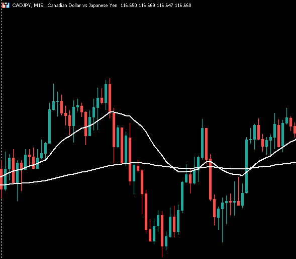
Fig 1: An example of moving average crossovers being applied on the CADJPY pair.
Overview
We're about to embark on an exciting journey where we'll link our MetaTrader5 terminal with our Python environment. First, we'll request M15 data for the EURUSD pair from January 1, 2020, to June 25, 2024. This extensive dataset will give us a comprehensive view of recent market behaviors.
Our next step is to establish two targets. The first will measure our accuracy in predicting direct price changes, serving as our baseline. This benchmark will help us compare how well we do when forecasting moving average crossovers. Along the way, we'll look for additional technical indicators to boost our accuracy. Finally, we'll ask our computer models to identify the key variables for predicting moving average crossovers. If the model doesn't prioritize the two moving averages we used, it might indicate that our initial assumptions were incorrect.
Before diving into the numbers, let's consider the possible outcomes:
-
Direct Price Prediction Superiority: If predicting price changes directly yields higher or equal accuracy compared to moving average crossovers, it suggests that forecasting crossovers might not provide any extra advantage, questioning the strategy's validity.
-
Crossover Prediction Superiority: If we achieve better accuracy in predicting moving average crossovers, it would motivate us to seek out more data to further enhance our predictions, highlighting the strategy's potential value.
-
Irrelevance of Moving Averages: If our models don't identify either moving average as crucial for forecasting crossovers, it implies other variables might be more significant, suggesting that the assumed relationship between the two moving averages doesn't hold.
-
Relevance of Moving Averages: If one or both moving averages are flagged as important for predicting crossovers, it confirms a substantial relationship between them, allowing us to build reliable models for informed predictions.
This analysis will help us understand the strengths and weaknesses of using moving average crossovers in our trading strategy, guiding us towards more effective forecasting methods.
The Experiment: Are Moving Average Crossovers Still Reliable?
Let us begin by first importing the standard Python libraries we need.
import pandas as pd
import pandas_ta as ta
import numpy as np
import MetaTrader5 as mt5
from   datetime import datetime
import seaborn as sns
import time
Next, we enter our login details.
account = 123436536
password = "Enter Your Password"
server = "Enter Your Broker"
Proceeding onwards, we will now attempt to log in to our trading account.
if(mt5.initialize(login=account,password=password,server=server)):
    print("Logged in succesfully")
else:
    print("Failed to login")
Logged in successfully
Next we will define a few global variables.
timeframe = mt5.TIMEFRAME_M15
deviation = 1000
volume = 0
lot_multiple = 10
symbol = "EURUSD"
Then we will fetch market data on the symbol we desire to trade.
#Setup trading volume
symbols = mt5.symbols_get()
for index,symbol in enumerate(symbols):
    if symbol.name == "EURUSD":
        print(f"{symbol.name} has minimum volume: {symbol.volume_min}")
        volume = symbol.volume_min * lot_multiple
EURUSD has minimum volume: 0.01
Now we will get ready to fetch training data.
#Specify date range of data to be modelled
date_start = datetime(2020,1,1)
date_end = datetime.now()
Next, we will define how far into the future we wish to forecast.
#Define how far ahead we are looking
look_ahead = 20
We can then proceed to fetch market data from our MetaTrader5 terminal, and then label the data. Our labelling scheme uses "1" to encode an up move and a "0" for down moves.
#Fetch market data
market_data = pd.DataFrame(mt5.copy_rates_range("EURUSD",timeframe,date_start,date_end))
market_data["time"] = pd.to_datetime(market_data["time"],unit='s')
#Add simple moving average technical indicator
market_data.ta.sma(length=5,append=True)
#Add simple moving average technical indicator
market_data.ta.sma(length=50,append=True)
#Delete missing rows
market_data.dropna(inplace=True)

#Add a column for the target
market_data["target"] = 0
market_data["close_target"] = 0

#Encoding the target
ma_cross_conditions = [
    (market_data["SMA_5"].shift(-look_ahead) > market_data["SMA_50"].shift(-look_ahead)),
    (market_data["SMA_5"].shift(-look_ahead) < market_data["SMA_50"].shift(-look_ahead))
]
#Encoding pattern
ma_cross_choices = [
    #Fast MA above Slow MA
    1,
    #Fast MA below Slow MA
    0
]

price_conditions = [
    (market_data["close"] > market_data["close"].shift(-look_ahead)),
    (market_data["close"] < market_data["close"].shift(-look_ahead))
]

#Encoding pattern
price_choices = [
    #Price fell
    0,
    #Price rose
    1
]

market_data["target"] = np.select(ma_cross_conditions,ma_cross_choices)
market_data["close_target"] = np.select(price_conditions,price_choices)

#The last rows do not have answers
market_data = market_data[:-look_ahead]
market_data
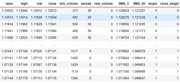
Fig 2: Our data frame with our market data in its current form.
We will now import the machine learning libraries we need.
#XGBoost
from xgboost import XGBClassifier
#Catboost
from catboost import CatBoostClassifier
#Random forest
from sklearn.ensemble import RandomForestClassifier
#LDA and QDA
from sklearn.discriminant_analysis import LinearDiscriminantAnalysis , QuadraticDiscriminantAnalysis
#Logistic regression
from sklearn.linear_model import LogisticRegression
#Neural network
from sklearn.neural_network import MLPClassifier
#Time series split
from sklearn.model_selection import TimeSeriesSplit
#Accuracy metrics
from sklearn.metrics import accuracy_score
#Visualising performance
from sklearn.metrics import confusion_matrix
import seaborn as sns
import matplotlib.pyplot as plt
from sklearn.model_selection import learning_curve
Getting ready to perform a time series split on the dataset.
#Time series split
splits = 10
gap = look_ahead
models = ["Logistic Regression","Linear Discriminant Analysis","Quadratic Discriminant Analysis","Random Forest Classifier","XGB Classifier","Cat Boost Classifier","Neural Network Small","Neural Network Large"]
We are going to assess the accuracy of many different models, and we will store the accuracy attained from each model in one data frame. One data frame will store our accuracy when forecasting moving average crossovers, and the second data frame measures our accuracy when forecasting changes in price directly.
error_ma_crossover = pd.DataFrame(index=np.arange(0,splits),columns=models)
error_price = pd.DataFrame(index=np.arange(0,splits),columns=models)
We will now proceed to measure the accuracy of each model. But first we must define the inputs our models will use.
predictors = ["open","high","low","close","tick_volume","spread","SMA_5","SMA_50"]
To measure the accuracy of each model, we will train our models on a fraction of the dataset and then test it on the remainder of the dataset that it didn't see during training. The TimeSeriesSplit library partitions our data frame for us and makes this process easier.
tscv = TimeSeriesSplit(n_splits=splits,gap=gap)
#Training each model to predict changes in the moving average cross over
for i,(train,test) in enumerate(tscv.split(market_data)):
    model = MLPClassifier(solver='lbfgs',alpha=1e-5,hidden_layer_sizes=(20, 10), random_state=1,early_stopping=True)
    model.fit( market_data.loc[train[0]:train[-1],predictors] , market_data.loc[train[0]:train[-1],"target"] )
    error_ma_crossover.iloc[i,7] = accuracy_score(market_data.loc[test[0]:test[-1],"target"],model.predict(market_data.loc[test[0]:test[-1],predictors]))
#Training each model to predict changes in the close price
for i,(train,test) in enumerate(tscv.split(market_data)):
    model = MLPClassifier(solver='lbfgs',alpha=1e-5,hidden_layer_sizes=(20, 10), random_state=1,early_stopping=True)
    model.fit( market_data.loc[train[0]:train[-1],predictors] , market_data.loc[train[0]:train[-1],"close_target"] )
    error_price.iloc[i,7] = accuracy_score(market_data.loc[test[0]:test[-1],"close_target"],model.predict(market_data.loc[test[0]:test[-1],predictors]))
Let us first see the data frame that measures our accuracy when forecasting changes in price directly.
error_price
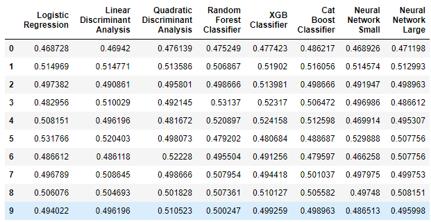
Fig 3: Our accuracy when forecasting changes in price directly.
Let's interpret the results before moving on. The first comment we can make is that none of the models we have are performing well on the task, some models demonstrated less than 50% accuracy when forecasting price directly. This performance is dismall, this imples that we could've performed more or less at par with these models by simply guessing randomly. Our models are arranged in order of increasing complexity, with simple logistic regression on the left and deep neural networks on the right. As we can observe, increasing the complexity of the models didn't increase our accuracy when forecasting price directly. Let us now see if there is any improvement when forecasting moving average crossovers instead.
error_ma_crossover
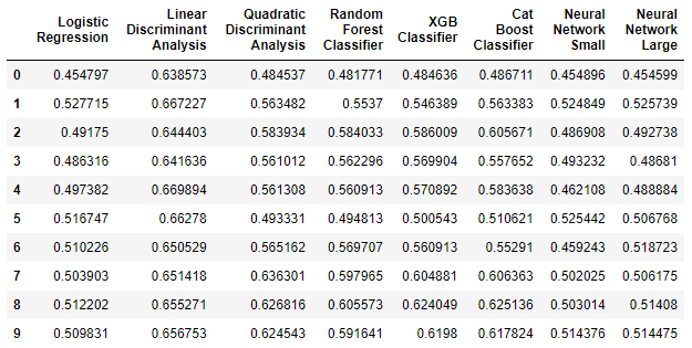
Fig 4: Our accuracy when forecasting moving average crossoevrs.
As we can see in the data frame above, Linear Discriminant Analysis (LDA) performed exceedingly well at this task. It was the best performing model we examined by a wide margin. Furthermore when you contrast the improved model performance of LDA with how poorly it performed the first task, we can clearly see that moving average crossovers may be more reliable to forecast than direct changes in price. The benefits of forecasting moving average crossovers cannot be disputed in such a case.
Visualising The Results
Let us visualise the results obtained above.
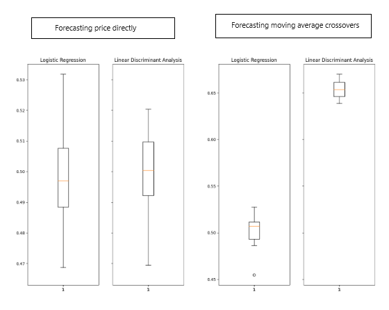
Fig 5: Visualising the results obtained.
The improvement in the LDA algorithm is notably visible in boxplots, indicating significant learning by our model. Additionally, there was a slight but noticeable enhancement in the performance of Logistic Regression. Notably, LDA consistently produced scores tightly clustered in boxplots when forecasting moving average crossovers, demonstrating desirable accuracy and consistency. This clustering suggests the model's predictions were stable, with likely stationary residuals indicating a reliable relationship learned by the model.
Now, let's analyze the types of errors our model made. We aim to determine whether it performs better in identifying upward movements, downward movements, or if its performance is balanced across both tasks.
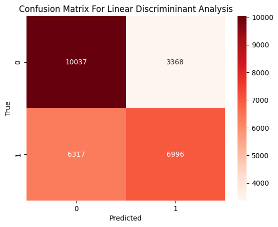
Fig 6: A confusion matrix of our LDA model performance.
The confusion matrix above displays the true classification on the left, and our model's prediction on the bottom. The data tells us that our model made more mistakes predicting up moves, it misclassified an up move as a down move 47% of the time. On the other hand, our model performed very well predicting down moves, our model only confused a true down move for an up move 25% of the time. Therefore, we can clearly see that our model is better at predicting down moves than it is at predicting up moves.
We can visualize the learning progress of our model as it encounters increasing amounts of training data. The plot below serves to assess whether our model is overfitting or underfitting the training data. Overfitting occurs when the model learns noise from the data, failing to capture meaningful relationships. Underfitting, on the other hand, is indicated by a significant gap between the training accuracy (represented by the blue line) and the validation accuracy (the orange line) on the plot. In our current plot, we observe a noticeable but not extensive gap between the training and validation scores, suggesting that our LDA model is indeed overfitting the training data. However, the scale on the left-hand side indicates that this overfitting is not severe.
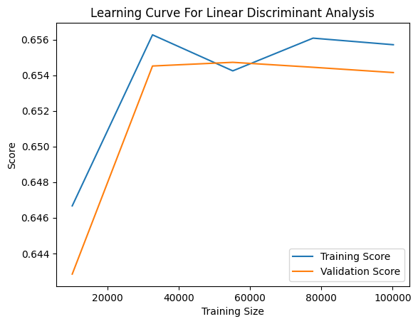
Fig 7: The learning curve for our LDA classifier.
On the other hand, underfitting is characterized by low training and validation accuracy. As an example, we've included the learning curve of one of our poorly performing models, the small neural network. In the plot below, we observe an unstable relationship between our model's performance and the amount of training data it has been exposed to. Initially, the model's validation performance deteriorates with increasing data, until it reaches a turning point and begins to improve as the training size approaches 10000 samples. Subsequently, the improvement plateaus, with only marginal enhancements despite large continued increases in the amount of training data available.
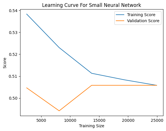
Fig 8: The learning curve for our small neural network.
Feature Elimination
In most machine learning projects, it's uncommon for all inputs to directly relate to the target variable. Typically, only a subset of available inputs are relevant to predicting the target. Eliminating irrelevant inputs offers several advantages, such as:
- Improved computational efficiency during model training and feature engineering.
- Enhanced model accuracy, especially if the removed features were noisy.
Next, we need to determine if there is a meaningful relationship between the moving averages. We'll employ feature elimination algorithms to validate the assumed relationship. If these algorithms fail to eliminate the moving averages from the input list, it indicates a meaningful relationship exists. Conversely, if they successfully remove these features, it suggests no significant relationship between the moving averages and the moving average crossover.
We will employ a feature selection technique known as backward selection. This method begins by fitting a linear model using all available inputs and then measuring the model's accuracy. Subsequently, one feature is removed at a time, and the impact on model accuracy is noted. The feature that causes the smallest decrease in accuracy is eliminated in each step until no features remain. At this stage, the algorithm automatically selects the most important features it has identified and recommends them for use.
One significant drawback of feature elimination worth mentioning is that when noisy and unimportant columns are present in our dataset, important columns may appear uninformative. Consequently, the backward selection algorithm might inadvertently eliminate an important feature because it appears uninformative due to the noise in the system.
Let us now proceed to see which columns our computer thinks are important. We start by importing a library called mlxtend that contains implementations of the backward selection algorithm.
from mlxtend.feature_selection import SequentialFeatureSelector
We then apply the algorithm on our dataset. Let's pay particular attention to 3 of the parameters we passed:
- "k_features=" instructs the algorithm on how many columns to select. We can instruct the algorithm to select only the columns it believes are necessary by passing an interval starting from 1 till the total number of columns in the dataset.
- "forward=" instructs the algorithm whether it should use forward or backward selection, we want to use backward selection therefore we set this parameter to "False".
- "n_jobs=" instructs the algorithm whether it should perform calculations in parallel, we pass "-1" to give the algorithm permission to use all available cores, this will reduce the amount of time spent significantly.
backward_feature_selector = SequentialFeatureSelector(LinearDiscriminantAnalysis(),
                                                      k_features=(1,market_data.loc[:,predictors].shape[1]),
                                                      forward=False,
                                                      verbose=2,
                                                      scoring="accuracy",
                                                      cv=5,
						      n_jobs=-1
                                                     ).fit(market_data.loc[:,predictors],market_data.loc[:,"target"])
[Parallel(n_jobs=-1)]: Using backend LokyBackend with 8 concurrent workers.
[Parallel(n_jobs=-1)]: Done 3 out of 8 | elapsed: 8.0s remaining: 13.3s
[Parallel(n_jobs=-1)]: Done 8 out of 8 | elapsed: 8.0s remaining: 0.0s
[Parallel(n_jobs=-1)]: Done 8 out of 8 | elapsed: 8.0s finished
Once the process is done, we can obtain a list of the inputs our algorithm thinks are important using the following command.
backward_feature_selector.k_feature_names_
('open', 'high', 'close', 'SMA_5', 'SMA_50')
And as we can see, the backward selection algorithm included our 2 moving averages in its list of important features. This is great news for us because it validates that our trading strategy is not just the result of a spurious regression.
Feature Engineering
Now that we've established a significant relationship between our two moving averages that warrants further improvement efforts, let's explore whether additional technical indicators can enhance our accuracy in forecasting moving average crossovers. This is where machine learning leans more towards art than science, as predicting which inputs will be beneficial beforehand is challenging. Our approach will involve adding several features we believe could be useful and assessing their actual impact.
We'll gather market data from the same market as before, but this time we'll incorporate additional indicators:
- Moving Average Convergence Divergence (MACD): The MACD is a very powerful trend confirming technical indicator that may help us better observe changes in underlying market regimes.
- Awesome Oscillator: The Awesome oscillator is renowned for providing very reliable exit signals, and it can clearly show us when any trend changes momentum.
- Aroon: The Aroon indicator is used to identify the beginning of new trends.
- Chaikins Commodity Index: The Chaikins Commodity Index acts as a barometer for measuring if a financial security is overbought or oversold.
- Percent Return: The Percent Return indicator helps us observe the growth in price and whether it is growing positively or negatively.
#Fetch market data
market_data = pd.DataFrame(mt5.copy_rates_range("EURUSD",timeframe,date_start,date_end))
market_data["time"] = pd.to_datetime(market_data["time"],unit='s')
#Add simple moving average technical indicator
market_data.ta.sma(length=5,append=True)
#Add simple moving average technical indicator
market_data.ta.sma(length=50,append=True)
#Add macd
market_data.ta.macd(append=True)
#Add awesome oscilator
market_data.ta.ao(append=True)
#Add aroon
market_data.ta.aroon(append=True)
#Add chaikins comodity index
market_data.ta.cci(append=True)
#Add percent return
market_data.ta.percent_return(append=True)
#Delete missing rows
market_data.dropna(inplace=True)
#Add the target
market_data["target"] = 0
market_data.loc[market_data["SMA_5"].shift(-look_ahead) > market_data["SMA_50"].shift(-look_ahead),"target"] = 1
market_data.loc[market_data["SMA_5"].shift(-look_ahead) < market_data["SMA_50"].shift(-look_ahead),"target"] = 0
#The last rows do not have answers
market_data = market_data[:-look_ahead]
market_data
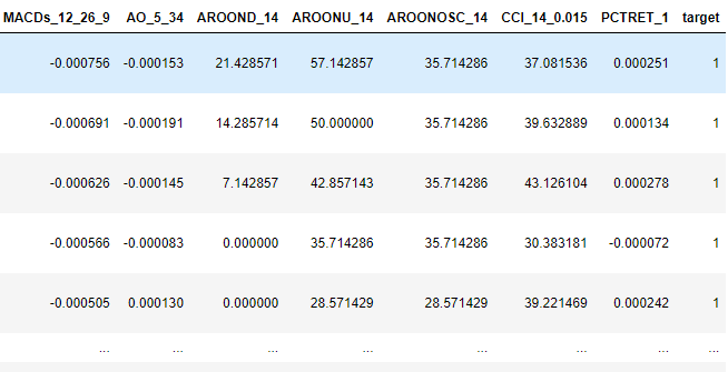
Fig 9: Some of the new additional rows we added to our data frame.
After conducting feature selection, our backward selection algorithm identified the following variables as important.
backward_feature_selector = SequentialFeatureSelector(LinearDiscriminantAnalysis(),
                                                      k_features=(1,market_data.loc[:,predictors].shape[1]),
                                                      forward=False,
                                                      verbose=2,
                                                      scoring="accuracy",
                                                      cv=5
                                                     ).fit(market_data.iloc[:,1:-1],market_data.loc[:,"target"])
backward_feature_selector.k_feature_names_
('close', 'tick_volume', 'spread', 'SMA_5', 'SMA_50', 'MACDh_12_26_9', 'AO_5_34')
Building Our Trading Strategy
Now we are ready to put everything we have learned so far into a consilidated trading strategy.
We first start by fitting our model on all the training data we have available, using only the columns we have identified are usefull.
predictors = ['close','tick_volume','spread','SMA_5','SMA_50','MACDh_12_26_9','AO_5_34']
model = LinearDiscriminantAnalysis()
model.fit(market_data.loc[:,predictors],market_data.loc[:,"target"])
Next we define functions for fetching market data from out MetaTrader5 terminal.
def get_prices():
    start = datetime(2024,6,1)
    end   = datetime.now()
    data  = pd.DataFrame(mt5.copy_rates_range("EURUSD",timeframe,start,end))
    #Add simple moving average technical indicator
    data.ta.sma(length=5,append=True)
    data.ta.sma(length=50,append=True)
    #Add awesome oscilator
    data.ta.ao(append=True)
    #Add macd
    data.ta.macd(append=True)
    #Delete missing rows
    data.dropna(inplace=True)
    data['time'] = pd.to_datetime(data['time'],unit='s')
    data.set_index('time',inplace=True)
    data = data.loc[:,['close','tick_volume','spread','SMA_5','SMA_50','MACDh_12_26_9','AO_5_34']]
    data = data.iloc[-2:,:]
    return(data)
Subsequently we need another method to get predictions from our LDA model.
#Get signals LDA model
def ai_signal(input_data,_model):
    #Get a forecast
    forecast = _model.predict(input_data)
    return forecast[1]
Now we can build our trading strategy.
#Now we define the main body of our Python Moving Average Crossover Trading Bot
if __name__ == '__main__':
    #We'll use an infinite loop to keep the program running
    while True:
        #Fetching model prediction
        signal = ai_signal(get_prices(),model)

        #Decoding model prediction into an action
        if signal == 1:
            direction = 'buy'
        elif signal == 0:
            direction = 'sell'

        print(f'AI Forecast: {direction}')

        #Opening A Buy Trade
        #But first we need to ensure there are no opposite trades open on the same symbol
        if direction == 'buy':
            #Close any sell positions
            for pos in mt5.positions_get():
                if pos.type == 1:
                    #This is an open sell order, and we need to close it
                    close_order(pos.ticket)

            if not mt5.positions_totoal():
                #We have no open positions
                mt5.Buy(symbol,volume)

        #Opening A Sell Trade
        elif direction == 'sell':
            #Close any buy positions
            for pos in mt5.positions_get():
                if pos.type == 0:
                    #This is an open buy order, and we need to close it
                    close_order(pos.ticket)

            if not mt5.positions_get():
                #We have no open positions
                mt5.sell(symbol,volume)

        print('time: ', datetime.now())
        print('-------\n')
        time.sleep(60)
AI Forecast: sell
time: 2024-06-25 14:35:37.954923
-------
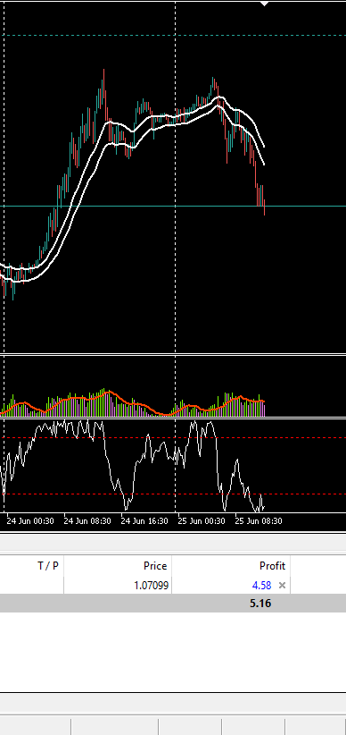
Fig 10: Our trading strategy in action.
Implementation In MQL5
Moving forward, let's utilize the MQL5 API to develop our own classifier from the ground up. There are numerous advantages to creating a custom classifier in MQL5. As the author, I firmly believe that native MQL5 solutions offer unparalleled flexibility.
If we were to export our model to ONNX format, we would need a separate model for each market we wish to trade. Additionally, trading across different time frames would require multiple ONNX models for each market. By building our classifier directly in MQL5, we gain the ability to trade any market without these limitations.
So let's create a new project.
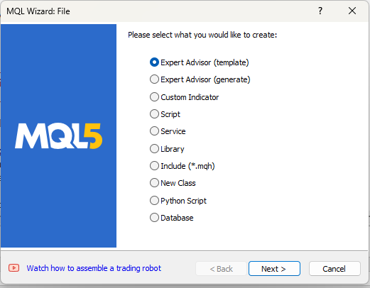
Fig 11: Creating an EA to implement our strategy.
Our first task is to define some global variables that we will use throughout our program.
//Global variables
int ma_5,ma_50;
double bid, ask;
double min_volume;
double ma_50_reading[],ma_5_reading[];
int size;
double current_prediction;
int state = -1;
matrix ohlc;
vector target;
double b_nort = 0;
double b_one = 0;
double b_two = 0;
long min_distance,atr_stop;
We will also have inputs that the end user can adjust.
//Inputs
int input lot_multiple = 20;
int input positions = 2;
double input sl_width = 0.4;
Lastly, we will import the trade library to help us manage our positions.
//Libraries
#include <Trade\Trade.mqh>
CTrade Trade;
Moving on, we need to define helper functions that will help us fetch data, label the training data, train our model and get predictions from our model. Let us start by defining a function to fetch training data and label the target for our classifier.
//+----------------------------------------------------------------------+
//|This function is responsible for getting our training data ready      |
//+----------------------------------------------------------------------+
void get_training_data(void)
  {
//How much data are we going to use?
   size = 100;
//Copy price data
   ohlc.CopyRates(_Symbol,PERIOD_CURRENT,COPY_RATES_CLOSE,1,size);
//Get indicator data
   ma_50 = iMA(_Symbol,PERIOD_CURRENT,50,0,MODE_EMA,PRICE_CLOSE);
   ma_5 = iMA(_Symbol,PERIOD_CURRENT,5,0,MODE_EMA,PRICE_CLOSE);
   CopyBuffer(ma_50,0,0,size,ma_50_reading);
   CopyBuffer(ma_5,0,0,size,ma_5_reading);
   ArraySetAsSeries(ma_50_reading,true);
   ArraySetAsSeries(ma_5_reading,true);
//Label the target
   target = vector::Zeros(size);
   for(int i = 0; i < size; i++)
     {
      if(ma_5_reading[i] > ma_50_reading[i])
        {
         target[i] = 1;
        }

      else
         if(ma_5_reading[i] < ma_50_reading[i])
           {
            target[i] = 0;
           }
     }

//Feedback
   Print("Done getting training data.");
  }
Our model has three coefficients it uses to make predictions. These coefficients need to be optimized. We'll use a beginner-friendly update equation to adjust these coefficients. By measuring the error in our model’s predictions, we will iteratively modify the coefficients to minimize the error and improve the accuracy of our system. But before we can start optmising the model, we need to first define how our model makes predicitons.
//+----------------------------------------------------------------------+
//|This function is responsible for making predictions using our model   |
//+----------------------------------------------------------------------+
double model_predict(double input_one,double input_two)
  {
//We simply return the probability that the shorter moving average will rise above the slower moving average
   double prediction = 1 / (1 + MathExp(-(b_nort + (b_one * input_one) + (b_two * input_two))));
   return prediction;
  }
Now that our model can make predictions, we can measure the error in its predictions and start the optimization process. Initially, all three coefficients will be set to 0. We will then iteratively adjust the coefficients in small steps to minimize the total error in our system.
//+----------------------------------------------------------------------+
//|This function is responsible for  training our model                  |
//+----------------------------------------------------------------------+
bool train_model(void)
  {
//Update the coefficients
   double learning_rate = 0.3;
   for(int i = 0; i < size; i++)
     {
      //Get a prediction from the model
      current_prediction = model_predict(ma_5_reading[i],ma_50_reading[i]);
      //Update each coefficient
      b_nort = b_nort + learning_rate * (target[i] - current_prediction) * current_prediction * (1 - current_prediction) * 1;
      b_one = b_one + learning_rate * (target[i] - current_prediction) * current_prediction * (1-current_prediction) * ma_5_reading[i];
      b_two = b_two + learning_rate * (target[i] - current_prediction) * current_prediction * (1-current_prediction) * ma_50_reading[i];
      Print(current_prediction);
     }

//Show updated coefficient values
   Print("Updated coefficient values");
   Print(b_nort);
   Print(b_one);
   Print(b_two);
   return(true);
  }
After successfully training the model, it would be beneficial to have a function that retrieves predictions from our model. These predictions will serve as our trading signals. Recall that a prediction of 1 is a buy signal, indicating that our model expects the shorter moving average to rise above the longer period moving average. Conversely, a prediction of 0 is a sell signal, indicating that our model expects the shorter moving average to fall below the longer moving average.
//Get the model's current forecast
void current_forecast()
  {
//Get indicator data
   ma_50 = iMA(_Symbol,PERIOD_CURRENT,50,0,MODE_EMA,PRICE_CLOSE);
   ma_5 = iMA(_Symbol,PERIOD_CURRENT,5,0,MODE_EMA,PRICE_CLOSE);
   CopyBuffer(ma_50,0,0,1,ma_50_reading);
   CopyBuffer(ma_5,0,0,1,ma_5_reading);
//Get model forecast
   model_predict(ma_5_reading[0],ma_50_reading[0]);
   interpret_forecast();
  }
We want our Expert Advisor to act based on the model's predictions. Therefore, we will write a function to interpret the model’s forecast and take the appropriate action: buy when the model predicts 1 and sell when the model predicts 0.
//+----------------------------------------------------------------------+
//|This function is responsible for taking action on our model's forecast|
//+----------------------------------------------------------------------+
void interpret_forecast(void)
  {
   if(current_prediction > 0.5)
     {
      state = 1;
      Trade.PositionOpen(_Symbol,ORDER_TYPE_BUY,min_volume * lot_multiple,ask,0,0,"Volatitlity Doctor AI");
     }

   if(current_prediction < 0.5)
     {
      state = 0;
      Trade.PositionOpen(_Symbol,ORDER_TYPE_SELL,min_volume * lot_multiple,bid,0,0,"Volatitlity Doctor AI");
     }
  }
Now that our application can learn from data, make predictions, and act on those predictions, we need to create additional functions to manage any open positions. Specifically, we want our program to add trailing stop losses and take profits to each position to manage our risk levels. We do not want to have open positions without a defined risk limit. Most trading strategies recommend a fixed stop loss size of 100 pips, but we want to ensure that our stop loss and take profit levels are dynamically placed based on current market volatility. Therefore, we will use the Average True Range (ATR) to calculate how wide or narrow our stops should be. We'll use a multiple of the ATR to determine these levels.
//+----------------------------------------------------------------------+
//|This function is responsible for calculating our SL & TP values       |
//+----------------------------------------------------------------------+
void CheckAtrStop()
  {

//First we iterate over the total number of open positions
   for(int i = PositionsTotal() -1; i >= 0; i--)
     {

      //Then we fetch the name of the symbol of the open position
      string symbol = PositionGetSymbol(i);

      //Before going any furhter we need to ensure that the symbol of the position matches the symbol we're trading
      if(_Symbol == symbol)
        {
         //Now we get information about the position
         ulong ticket = PositionGetInteger(POSITION_TICKET); //Position Ticket
         double position_price = PositionGetDouble(POSITION_PRICE_OPEN); //Position Open Price
         long type = PositionGetInteger(POSITION_TYPE); //Position Type
         double current_stop_loss = PositionGetDouble(POSITION_SL); //Current Stop loss value

         //If the position is a buy
         if(type == POSITION_TYPE_BUY)
           {

            //The new stop loss value is just the ask price minus the ATR stop we calculated above
            double atr_stop_loss = NormalizeDouble(ask - ((min_distance * sl_width)/2),_Digits);
            //The new take profit is just the ask price plus the ATR stop we calculated above
            double atr_take_profit = NormalizeDouble(ask + (min_distance * sl_width),_Digits);

            //If our current stop loss is less than our calculated ATR stop loss
            //Or if our current stop loss is 0 then we will modify the stop loss and take profit
            if((current_stop_loss < atr_stop_loss) || (current_stop_loss == 0))
              {
               Trade.PositionModify(ticket,atr_stop_loss,atr_take_profit);
              }
           }

         //If the position is a sell
         else
            if(type == POSITION_TYPE_SELL)
              {
               //The new stop loss value is just the ask price minus the ATR stop we calculated above
               double atr_stop_loss = NormalizeDouble(bid + ((min_distance * sl_width)/2),_Digits);
               //The new take profit is just the ask price plus the ATR stop we calculated above
               double atr_take_profit = NormalizeDouble(bid - (min_distance * sl_width),_Digits);

               //If our current stop loss is greater than our calculated ATR stop loss
               //Or if our current stop loss is 0 then we will modify the stop loss and take profit
               if((current_stop_loss > atr_stop_loss) || (current_stop_loss == 0))
                 {
                  Trade.PositionModify(ticket,atr_stop_loss,atr_take_profit);
                 }
              }
        }
     }
  }
Then we need a function that we will call whenever we want to calculate new stop loss and take profit values.
//+------------------------------------------------------------------+
//|This function is responsible for updating our SL&TP values        |
//+------------------------------------------------------------------+
void ManageTrade()
  {
   CheckAtrStop();
  }
Now that we have defined our helper functions, we can start calling them within our event handlers. When our program loads for the first time, we want to initiate the training process. Therefore, we will call our helper function responsible for training our expert inside the OnInit event handler.
//+------------------------------------------------------------------+
//| Expert initialization function                                   |
//+------------------------------------------------------------------+
int OnInit()
  {
   //Define important global variables
   min_volume = SymbolInfoDouble(_Symbol,SYMBOL_VOLUME_MIN);
   min_distance = SymbolInfoInteger(_Symbol,SYMBOL_TRADE_STOPS_LEVEL);
   //Train the model
   get_training_data();
   if(train_model())
     {
      interpret_forecast();
     }
   return(INIT_SUCCEEDED);
  }
After training the model, we can start actual trading.
//+------------------------------------------------------------------+
//| Expert tick function                                             |
//+------------------------------------------------------------------+
void OnTick()
  {
//Get updates bid and ask prices
   bid = SymbolInfoDouble(_Symbol,SYMBOL_BID);
   ask = SymbolInfoDouble(_Symbol,SYMBOL_ASK);

   if(PositionsTotal() == 0)
     {
      current_forecast();
     }

   if(PositionsTotal() > 0)
     {
      ManageTrade();
     }
  }
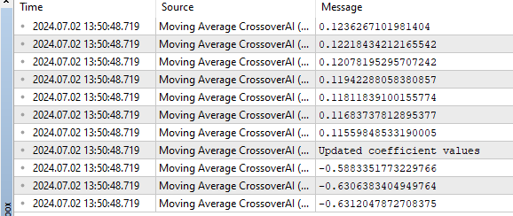
Fig 12: A sample of the ouput from our Expert Advisor.
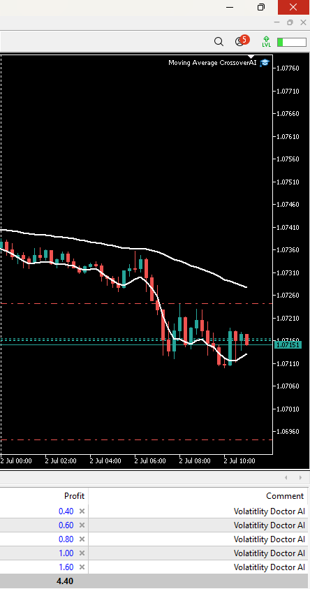
Fig 13: Our expert advisor in action.
Conclusion
In this article, we have demonstrated that it is computationally easier for our model to predict moving average crossovers than to predict changes in price directly.
As with all my articles, I prefer to provide technical explanations at the end, while demonstrating the principle first. There are several possible reasons for this observation. One potential reason is that, depending on the chosen periods, moving averages may not cross over as frequently as prices change direction erratically. In other words, over the past two hours, the price may have gone up, then down, or changed direction twice. However, during that same period, the moving averages might not have crossed over at all. Therefore, moving average crossovers may be easier to forecast because they do not change direction as rapidly as the price itself does. This is just one possible explanation. Feel free to think for yourself, draw your own conclusions, and share them in the comments below.
Moving forward, we employed backward selection for feature elimination, a technique where a linear model is iteratively trained with one feature removed at each step based on its impact on model accuracy. This approach helps identify and retain the most informative features, although it's susceptible to eliminating important features that may appear uninformative due to noise.
Having validated a significant relationship between two moving averages, we explored integrating additional technical indicators: MACD, Awesome Oscillator, Aroon, Chaikins Commodity Index, and Percent Return. These indicators aim to enhance our ability to forecast moving average crossovers accurately. However, the selection of these indicators remains somewhat of an art due to the unpredictable nature of their impact on model performance.
Overall, our approach blends empirical validation with strategic feature selection to quantitatively prove that indeed moving averages crossovers can be predicted and furthermore any effort spent trying to improve this trading strategy would emphatically not be a waste of time.
 Sentiment Analysis and Deep Learning for Trading with EA and Backtesting with Python
 Neural networks made easy (Part 77): Cross-Covariance Transformer (XCiT)
 MQL5 Wizard Techniques you should know (Part 26): Moving Averages and the Hurst Exponent
 Building A Candlestick Trend Constraint Model (Part 5): Notification System (Part III)
- Free trading apps
- Over 8,000 signals for copying
- Economic news for exploring financial markets
You agree to website policy and terms of use
Any assistance with this error
The 'sklearn' PyPI package is deprecated, use 'scikit-learn'
rather than 'sklearn' for pip commands.
Any assistance with this error
The 'sklearn' PyPI package is deprecated, use 'scikit-learn'
rather than 'sklearn' for pip commands.