
Neural Networks Made Easy (Part 81): Context-Guided Motion Analysis (CCMR)

Introduction
As part of this series, we became acquainted with various methods for analyzing the state of the environment and algorithms for using the obtained data. We used convolutional models to find stable patterns in historical price movement data. We also used attention models to find dependencies between distinct local environmental states. We always assessed the state of the environment as a certain cross-section at a point in time. However, we have never assessed the dynamics of environmental indicators. We assumed that the model, in the process of analyzing and comparing environmental conditions, would somehow pay attention to key changes. But we did not use an explicit quantitative representation of such dynamics.
However, in the field of computer vision, there is a fundamental problem of optical flow estimation. The solution to this problem provides information about the movement of objects in the scene. To solve this problem, a number of interesting algorithms have been proposed and are now widely used. Optical flow estimation results are used in various fields from autonomous driving to object tracking and surveillance.
Most current approaches use convolutional neural networks, but they lack global context. This makes it difficult to reason about object occlusions or large displacements. An alternative approach is to use transformers and other attention techniques. They allow you to go far beyond the fixed receptive field of classical CNNs.
A particularly interesting method entitled CCMR was presented in the paper "CCMR: High Resolution Optical Flow Estimation via Coarse-to-Fine Context-Guided Motion Reasoning". It is an approach to optical flow estimation that combines the advantages of attention-oriented methods of motion aggregation concepts and high-resolution multi-scale approaches. The CCMR method consistently integrates context-based motion grouping concepts into a high-resolution coarse-grained estimation framework. This allows for detailed flow fields that also provide high accuracy in occluded areas. In this context, the authors of the method propose a two-stage motion grouping strategy where global self-attentional contextual features are first computed and them used to guide motion features iteratively across all scales. Thus, context-directed reasoning about XCiT-based motion provides processing at all coarse-grained scales. Experiments conducted by the authors of the method demonstrate the strong performance of the proposed approach and the advantages of its basic concepts.
1. The CCMR algorithm
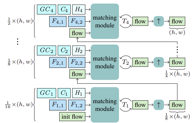
The CCMR method estimates optical flow using recurrent updates at coarse and fine scales using a common Gated Recurrent Unit (GRU). Before starting with the estimation, for each scale S, features Fs,1, Fs,2 are computed for matching. In addition, context features Cs and, based on them, global context features GCs are computed, as well as the initial hidden state Hs for the current scale of the recurrent block from the reference state I1.
Starting from the coarsest scale of 1/16, the flow is computed based on the above features F1,1, F1,2, C1, GC1, H1. After T1 recurrent flow updates, the estimated flow is upsampled using a shared X2 convex upsampler, where the flow serves as an initialization for the matching process at the next finer scale. This process continues until the flow is computed at the finest 1/2 scale and upsampled to the original resolution.
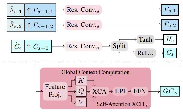
The authors of the method proposed to extract multi-scale image and context features using a feature extractor. To do this, intermediate features are computed from top to bottom, and then, to obtain multi-scale features, more structured and finer features Fs,1,Fs,2 and Cs are semantically boosted by combining them with deeper coarser-scale features Fs−1,1,Fs−1,2 and Cs−1 for S∈ {2, 3, 4}. Thus, consolidation is performed by stacking the upsampled coarser features and intermediate finer features and their aggregation.
Based on the multi-scale Cs context features, global context features are computed. Here the goal is to obtain more meaningful features, which are then used to control motion. To do this, aggregation of contextual features Cs is performed using channel statistics using the XCiT layer, which ensures linear complexity with respect to the number of tokens. This architectural choice allows for possible context aggregation at all coarse and fine scales during estimation. It is important to note that the authors' proposed CCMR approach to using XCiT is different from its original approach, where the XCiT layer is actually applied to a coarser representation of its input data, implemented through explicit patching, and then upsampled again to the original resolution. Within CCMR, in contrast, the XCiT layer is applied directly to features at all coarse and fine scales using scale-specific content. To compute global context, positional coding is first added to context features Cs. Then the layer is normalized. At this stage, to implement Self-Attention, all Query, Key and Value features are computed from Csp. Before applying the cross-covariance attention step, channels KCs, QCs, VCs are reshaped into h heads. The cross-covariance attention is then calculated as XCA(KCs, QCs, VCs). After that, a local patch interaction layer (LPI) and then the FFN block is applied.
While cross-covariance attention provides global interactions between channels in each head, the LPI and FFN modules provide explicit spatial interactions between tokens locally and connections between all channels, respectively.
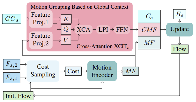
First, based on the initial flow in the first iteration (or the updated flow in subsequent iterations), the neighborhood matching costs are calculated from the image features (Fs,1, Fs,2). The calculated costs, along with the current flow estimate, are then processed through a motion encoder, which outputs motion features that are ultimately used by the GRU to compute a thread update.
When computing iterative flow updates, incorporating globally aggregated motion features based on contextual features can help resolve ambiguities in occluded regions. This is logical because the movement of occluded pixels from a partially unoccluded object can usually be inferred from the movement of its unoccluded pixels. To aggregate motion features in a single scale setting, the authors of the method follow their efficient strategy based on global channel statistics from the global context calculation, which is performed at all coarse and fine scales. Motion grouping is performed using a cross-attention layer XCiT applied to global contextual features GCs and movement features MF. Thus, we calculate Query and Key from global contextual features GCs and Value from motion features directly at each scale without explicit partitioning into patches. After applying XCA, LPI, and FFN to the context's Query, Key, and Value, the context-driven motion features (CMFs), context-driven motion features Cs, and initial motion features MFs are combined and passed through a recurrent block to iteratively compute the update flow.
Note that using token cross-attention to perform motion aggregation in coarse-grained and fine-tuned schemes is not practical in terms of memory usage.
The original visualization of the CCMR method presented by its authors is provided below.
2. Implementation using MQL5
After considering the theoretical aspects of the CCMR method, we move on to the practical part of our article, in which we implement the proposed approaches using MQL5. As you can see, the proposed architecture is quite complex. Therefore, I decided to divide the implementation of the proposed algorithms into several blocks.
2.1 Closed-loop convolutional block
We will start with the closed-loop convolutional block. To implement it, let's create class CResidualConv, which will inherit the basic functionality from the fully connected layer class CNeuronBaseOCL.
The structure of the new class is shown below. As you can see, it contains a familiar set of methods.
class CResidualConv  :  public CNeuronBaseOCL
  {
protected:
   int               iWindowOut;
   //---
   CNeuronConvOCL    cConvs[3];
   CNeuronBatchNormOCL cNorm[3];
   CNeuronBaseOCL    cTemp;
   //---
   virtual bool      feedForward(CNeuronBaseOCL *NeuronOCL);
   virtual bool      updateInputWeights(CNeuronBaseOCL *NeuronOCL);

public:
                     CResidualConv(void) {};
                    ~CResidualConv(void) {};
   //---
   virtual bool      Init(uint numOutputs, uint myIndex, COpenCLMy *open_cl,
                          uint window, uint window_out, uint count,
                          ENUM_OPTIMIZATION optimization_type,
                          uint batch);
   virtual bool      calcInputGradients(CNeuronBaseOCL *prevLayer);
   //---
   virtual int       Type(void)   const   {  return defResidualConv;   }
   //--- methods for working with files
   virtual bool      Save(int const file_handle);
   virtual bool      Load(int const file_handle);
   virtual CLayerDescription* GetLayerInfo(void);
   virtual void      SetOpenCL(COpenCLMy *obj);
   virtual void      TrainMode(bool flag);                ///< Set Training Mode Flag
  };
The class functionality will use 3 blocks of a convolutional layer and batch normalization. All internal layers are declared static, which allows us to leave the class constructor and destructor empty.
Initialization of a class object is performed in the Init method. In the method parameters, we will pass constants that define the architecture of the class.
bool CResidualConv::Init(uint numOutputs, uint myIndex, COpenCLMy *open_cl,
                         uint window, uint window_out, uint count,
                         ENUM_OPTIMIZATION optimization_type, uint batch)
  {
   if(!CNeuronBaseOCL::Init(numOutputs, myIndex, open_cl, window_out * count, optimization_type, batch))
      return false;
In the body of the method, we use the same name method of the parent class to control the received parameters and initialize inherited objects.
After the parent class method successfully executes, we initialize the internal objects.
   if(!cConvs[0].Init(0, 0, OpenCL, window, window, window_out, count, optimization, iBatch))
      return false;
   if(!cNorm[0].Init(0, 1, OpenCL, window_out * count, iBatch, optimization))
      return false;
   cNorm[0].SetActivationFunction(LReLU);
To extract features from the analyzed state of the environment, we use 2 blocks of sequential convolutional layer and batch normalization with LReLU function to create nonlinearity between them.
   if(!cConvs[1].Init(0, 2, OpenCL, window_out, window_out, window_out, count, optimization, iBatch))
      return false;
   if(!cNorm[1].Init(0, 3, OpenCL, window_out * count, iBatch, optimization))
      return false;
   cNorm[1].SetActivationFunction(None);
We use the third block of convolutional layer and batch normalization (without activation function) to scale the original data to the size of results of our CResidualConv. This will allow us to implement a second data flow.
   if(!cConvs[2].Init(0, 4, OpenCL, window, window, window_out, count, optimization, iBatch))
      return false;
   if(!cNorm[2].Init(0, 5, OpenCL, window_out * count, iBatch, optimization))
      return false;
   cNorm[2].SetActivationFunction(None);
Creating 2 parallel data flows obliges us to transmit the error gradient in similar parallel flows. We use an auxiliary inner layer to sum the error gradients.
   if(!cTemp.Init(0, 6, OpenCL, window * count, optimization, batch))
      return false;
To avoid unnecessary data copying, we replace data buffers.
   cNorm[1].SetGradientIndex(getGradientIndex());
   cNorm[2].SetGradientIndex(getGradientIndex());
   SetActivationFunction(None);
   iWindowOut = (int)window_out;
//---
   return true;
  }
We implement the feed-forward functionality in the CResidualConv::feedForward method. In the method parameters, we receive a pointer to the previous neural layer.
bool CResidualConv::feedForward(CNeuronBaseOCL *NeuronOCL)
  {
//---
   if(!cConvs[0].FeedForward(NeuronOCL))
      return false;
   if(!cNorm[0].FeedForward(GetPointer(cConvs[0])))
      return false;
In the body of the method, we do not organize a check of the received pointer, since such a check is already implemented in the relevant methods of the internal layers. Therefore, we immediately proceed to calling feed-forward methods for internal layers.
   if(!cConvs[1].FeedForward(GetPointer(cNorm[0])))
      return false;
   if(!cNorm[1].FeedForward(GetPointer(cConvs[1])))
      return false;
As mentioned above, we use the data received from the previous neural layer for the feed-forward pass of blocks 1 and 3.
   if(!cConvs[2].FeedForward(NeuronOCL))
      return false;
   if(!cNorm[2].FeedForward(GetPointer(cConvs[2])))
      return false;
Then we add and normalize their results.
   if(!SumAndNormilize(cNorm[1].getOutput(), cNorm[2].getOutput(), Output, iWindowOut, true))
      return false;
//---
   return true;
  }
The reverse process of error gradient backpropagation is implemented in the CResidualConv::calcInputGradients method. Its algorithm is quite similar to the feed-forward method. We just call the methods of the same name on the internal layers, but in the reverse order.
bool CResidualConv::calcInputGradients(CNeuronBaseOCL *prevLayer)
  {
   if(!cNorm[2].calcInputGradients(GetPointer(cConvs[2])))
      return false;
   if(!cConvs[2].calcInputGradients(GetPointer(cTemp)))
      return false;
//---
   if(!cNorm[1].calcInputGradients(GetPointer(cConvs[1])))
      return false;
   if(!cConvs[1].calcInputGradients(GetPointer(cNorm[0])))
      return false;
   if(!cNorm[0].calcInputGradients(prevLayer))
      return false;
You should note here that by replacing data buffers, we eliminated the initial copying of error gradients to internal layers. To the previous layer, we transfer the sum of error gradients from 2 data flows.
   if(!SumAndNormilize(prevLayer.getGradient(), cTemp.getGradient(), prevLayer.getGradient(), iWindowOut, false))
      return false;
//---
   return true;
  }
The CResidualConv::updateInputWeights method for updating class parameters is organized similarly. I suggest you familiarize yourself with it using the attached code. The full code of the CResidualConv class and all its methods is attached below. The attachment also include complete code for all programs used while preparing the article. We now move on to considering the algorithm for constructing the next block: the Feature Encoder.
2.2 The Feature Encoder
The Feature Encoder algorithm proposed by the authors of the CCMR method will be implemented in the CCCMREncoder class, which also inherits from the base class of the fully connected neural layer CNeuronBaseOCL.
class CCCMREncoder   :  public CNeuronBaseOCL
  {
protected:
   CResidualConv     cResidual[6];
   CNeuronConvOCL    cInput;
   CNeuronBatchNormOCL cNorm;
   CNeuronConvOCL    cOutput;
   //---
   virtual bool      feedForward(CNeuronBaseOCL *NeuronOCL);
   virtual bool      updateInputWeights(CNeuronBaseOCL *NeuronOCL);

public:
                     CCCMREncoder(void) {};
                    ~CCCMREncoder(void) {};
   //---
   virtual bool      Init(uint numOutputs, uint myIndex, COpenCLMy *open_cl,
                          uint window, uint window_out, uint count,
                          ENUM_OPTIMIZATION optimization_type,
                          uint batch);
   //---
   virtual bool      calcInputGradients(CNeuronBaseOCL *prevLayer);
   //---
   virtual int       Type(void)   const   {  return defCCMREncoder;   }
   //--- methods for working with files
   virtual bool      Save(int const file_handle);
   virtual bool      Load(int const file_handle);
   virtual CLayerDescription* GetLayerInfo(void);
   virtual void      SetOpenCL(COpenCLMy *obj);
   virtual void      TrainMode(bool flag);                ///< Set Training Mode Flag
  };
In this class, we use a convolutional layer to project the original data cInput, the results of which we normalize with the batch normalization layer cNorm. We also use the convolutional layer of the Encoder's operation results projection cOutput. Since we use a projection layer of the source data and the results, we can set up cascaded feature extraction at several scales without reference to the size of the source data and the desired number of features.
Data scaling and feature extraction processes are performed in several sequential closed-loop convolutional blocks, which for convenience we have combined into the array cResidual.
As in the previous class, we declared all internal objects of the class static, which allows us to leave the constructor and destructor of the class empty.
Initialization of class objects is performed in the CCCMREncoder::Init method. The algorithm of this method follows an already familiar logic. In parameters, the method receives class architecture constants.
bool CCCMREncoder::Init(uint numOutputs, uint myIndex, COpenCLMy *open_cl,
                        uint window, uint window_out, uint count,
                        ENUM_OPTIMIZATION optimization_type, uint batch)
  {
   if(!CNeuronBaseOCL::Init(numOutputs, myIndex, open_cl, window_out * count, optimization_type, batch))
      return false;
In the body of the method, we first call the relevant method of the parent class, which checks the received parameters and initializes the inherited objects. We control the result of the parent class method using the logical result of its completion.
Next, we initialize the block for scaling and normalizing the source data. Based on the results of its operation, we plan to obtain a representation of a single state of the environment in the form of a description of 32 parameters.
   if(!cInput.Init(0, 0, OpenCL, window, window, 32, count, optimization, iBatch))
      return false;
   if(!cNorm.Init(0, 1, OpenCL, 32 * count, iBatch, optimization))
      return false;
   cNorm.SetActivationFunction(LReLU);
We then create a data scaling cascade with the number of features {32, 64, 128}.
   if(!cResidual[0].Init(0, 2, OpenCL, 32, 32, count, optimization, iBatch))
      return false;
   if(!cResidual[1].Init(0, 3, OpenCL, 32, 32, count, optimization, iBatch))
      return false;
   if(!cResidual[2].Init(0, 4, OpenCL, 32, 64, count, optimization, iBatch))
      return false;
   if(!cResidual[3].Init(0, 5, OpenCL, 64, 64, count, optimization, iBatch))
      return false;
   if(!cResidual[4].Init(0, 6, OpenCL, 64, 128, count, optimization, iBatch))
      return false;
   if(!cResidual[5].Init(0, 7, OpenCL, 128, 128, count, optimization, iBatch))
      return false;
And finally, we bring the data dimension to the scale specified by the user.
   if(!cOutput.Init(0, 8, OpenCL, 128, 128, window_out, count, optimization, iBatch))
      return false;
To eliminate unnecessary copying operations of block operation results and error gradients, we replace data buffers.
   if(Output != cOutput.getOutput())
     {
      if(!!Output)
         delete Output;
      Output = cOutput.getOutput();
     }
//---
   if(Gradient != cOutput.getGradient())
     {
      if(!!Gradient)
         delete Gradient;
      Gradient = cOutput.getGradient();
     }
//---
   return true;
  }
Do not forget to control the process of operations at every step. Then we inform the caller about the method results with a logical value.
Now we create a feed-forward pass algorithm in the CCCMREncoder::feedForward method. In the method parameters, as always, we receive a pointer to the object of the previous layer. Checking the relevance of the received pointer is carried out in the body of methods for the feed-forward pass of nested objects.
bool CCCMREncoder::feedForward(CNeuronBaseOCL *NeuronOCL)
  {
   if(!cInput.FeedForward(NeuronOCL))
      return false;
   if(!cNorm.FeedForward(GetPointer(cInput)))
      return false;
First, we scale and normalize the original data. Then we will put the data through a scaling cascade with feature extraction.
Note that the first closed-loop convolutional block receives its initial data from the batch normalization layer, and the subsequent ones from the previous block from the array. This allows us to iterate through blocks in a loop.
   if(!cResidual[0].FeedForward(GetPointer(cNorm)))
      return false;
   for(int i = 1; i < 6; i++)
      if(!cResidual[i].FeedForward(GetPointer(cResidual[i - 1])))
         return false;
We scale the result of the operations to a given size.
   if(!cOutput.FeedForward(GetPointer(cResidual[5])))
      return false;
//---
   return true;
  }
The error gradient is propagated through internal Encoder objects in the reverse order.
bool CCCMREncoder::updateInputWeights(CNeuronBaseOCL *NeuronOCL)
  {
   if(!cInput.UpdateInputWeights(NeuronOCL))
      return false;
   if(!cNorm.UpdateInputWeights(GetPointer(cInput)))
      return false;
   if(!cResidual[0].UpdateInputWeights(GetPointer(cNorm)))
      return false;
   for(int i = 1; i < 6; i++)
      if(!cResidual[i].UpdateInputWeights(GetPointer(cResidual[i - 1])))
         return false;
   if(!cOutput.UpdateInputWeights(GetPointer(cResidual[5])))
      return false;
//---
   return true;
  }
In this article, we will not dwell in more detail on the description of all the methods of the class. They have a similar block structure of sequential calling of the corresponding methods of internal objects. You can study the structure using the complete code attached below. If you have any questions regarding the code, I will be happy to answer them on the forum or in private messages. Choose your preferred communication format.
2.3 Dynamic grouping of global context
To group the global context taking into account the dynamics of changes in features, the authors of the CCRM method proposed using a cross-attention block XCiT. In this block, the Query and Key entities are formed from features of the global context. Value is formed from the dynamics of the formed environmental features of 2 subsequent states. This use of the block is somewhat different from the one we considered previously. To implement the proposed option for using the block, we need to make some modifications.
Let's create a new class CNeuronCrossXCiTOCL, which will inherit most of the functionality from the previous implementation of the XCiT method.
class CNeuronCrossXCiTOCL  :  public CNeuronXCiTOCL
  {
protected:
   CCollection       cConcat;
   CCollection       cValue;
   CCollection       cV_Weights;
   CBufferFloat      TempBuffer;
   uint              iWindow2;
   //---
   virtual bool      feedForward(CNeuronBaseOCL *NeuronOCL, CBufferFloat *Motion);
   virtual bool      Concat(CBufferFloat *input1, CBufferFloat *input2, CBufferFloat *output,
                            int window1, int window2);
   //---
   virtual bool      updateInputWeights(CNeuronBaseOCL *NeuronOCL, CBufferFloat *Motion);
   virtual bool      DeConcat(CBufferFloat *input1, CBufferFloat *input2, CBufferFloat *output,
                              int window1, int window2);

public:
                     CNeuronCrossXCiTOCL(void) {};
                    ~CNeuronCrossXCiTOCL(void) {};
   //---
   virtual bool      Init(uint numOutputs, uint myIndex, COpenCLMy *open_cl,
                          uint window1, uint window2, uint lpi_window, uint heads,
                          uint units_count, uint layers,
                          ENUM_OPTIMIZATION optimization_type,
                          uint batch);
   virtual bool      calcInputGradients(CNeuronBaseOCL *prevLayer, CNeuronBaseOCL *Motion);
   //---
   virtual int       Type(void)   const   {  return defNeuronCrossXCiTOCL;   }
   //--- methods for working with files
   virtual bool      Save(int const file_handle);
   virtual bool      Load(int const file_handle);
   virtual CLayerDescription* GetLayerInfo(void);
   virtual void      SetOpenCL(COpenCLMy *obj);
  };
Note that in this implementation, I tried to use the previously created functionality to the maximum. 3 collections of data buffers and one auxiliary buffer for storing intermediate data were added to the class structure.
As before, all internal objects are declared static, so the class constructor and destructor are "empty".
Initialization of all class objects is performed in the method CNeuronCrossXCiTOCL::Init.
bool CNeuronCrossXCiTOCL::Init(uint numOutputs, uint myIndex, COpenCLMy *open_cl,
                               uint window1, uint window2, uint lpi_window,
                               uint heads, uint units_count, uint layers,
                               ENUM_OPTIMIZATION optimization_type, uint batch)
  {
   if(!CNeuronXCiTOCL::Init(numOutputs, myIndex, open_cl, window1, lpi_window,
                            heads, units_count, layers, optimization_type, batch))
      return false;
In the parameters, the method receives the main parameters that determine the architecture of the entire class and its internal objects. In the body of the class, we call the relevant method of the parent class, which checks the received parameters and initializes all inherited objects.
After successful execution of the parent class method, we define the parameters of the buffers for writing Value entities and their error gradients. We also define weight generation matrices for the specified entity.
//--- Cross XCA
   iWindow2 = fmax(window2, 1);
   uint num = iWindowKey * iHeads * iUnits;                 //Size of V tensor
   uint v_weights = (iWindow2 + 1) * iWindowKey * iHeads;   //Size of weights' matrix of V tensor
Next, we organize a loop by the number of XCiT cross-attention internal layers and create the required buffers in the body of the loop. We first add a buffer to write the generated Value entities and the corresponding error gradients.
   for(uint i = 0; i < iLayers; i++)
     {
      CBufferFloat *temp = NULL;
      for(int d = 0; d < 2; d++)
        {
         //--- XCiT
         //--- Initilize V tensor
         temp = new CBufferFloat();
         if(CheckPointer(temp) == POINTER_INVALID)
            return false;
         if(!temp.BufferInit(num, 0))
            return false;
         if(!temp.BufferCreate(OpenCL))
            return false;
         if(!cValue.Add(temp))
            return false;
In the parent class CNeuronXCiTOCL, we used a concatenated buffer of Query, Key and Value entities. In order to be able to further use the inherited functionality, let's concatenate the specified entities from 2 sources into one cConcat collection buffer.
         //--- Initilize QKV tensor
         temp = new CBufferFloat();
         if(CheckPointer(temp) == POINTER_INVALID)
            return false;
         if(!temp.BufferInit(3 * num, 0))
            return false;
         if(!temp.BufferCreate(OpenCL))
            return false;
         if(!cConcat.Add(temp))
            return false;
        }
The next step is to create the weight matrix buffers to generate the Value entity.
      //--- XCiT
      //--- Initilize V weights
      temp = new CBufferFloat();
      if(CheckPointer(temp) == POINTER_INVALID)
         return false;
      if(!temp.Reserve(v_weights))
         return false;
      float k = (float)(1 / sqrt(iWindow + 1));
      for(uint w = 0; w < v_weights; w++)
        {
         if(!temp.Add((GenerateWeight() - 0.5f)* k))
            return false;
        }
      if(!temp.BufferCreate(OpenCL))
         return false;
      if(!cV_Weights.Add(temp))
         return false;
Moment buffers for the optimization process of the specified weight matrix.
      for(int d = 0; d < (optimization == SGD ? 1 : 2); d++)
        {
         //--- XCiT
         temp = new CBufferFloat();
         if(CheckPointer(temp) == POINTER_INVALID)
            return false;
         if(!temp.BufferInit(v_weights, 0))
            return false;
         if(!temp.BufferCreate(OpenCL))
            return false;
         if(!cV_Weights.Add(temp))
            return false;
        }
     }
Then we initialize the intermediate data storage buffer.
   TempBuffer.BufferInit(iWindow2 * iUnits, 0);
   if(!TempBuffer.BufferCreate(OpenCL))
      return false;
//---
   return true;
  }
Do not forget to control the process of operations at every step.
The feed-forward method CNeuronCrossXCiTOCL::feedForward was largely copied from the parent class. However, the cross-attention features require its redefinition. In particular, to implement cross-attention, we need two sources of initial data.
bool CNeuronCrossXCiTOCL::feedForward(CNeuronBaseOCL *NeuronOCL, CBufferFloat *Motion)
  {
   if(!NeuronOCL || !Motion)
      return false;
In the body of the method, we check the relevance of the received pointers to the source data objects and organize a loop through the internal layers.
   for(uint i = 0; (i < iLayers && !IsStopped()); i++)
     {
      //--- Calculate Queries, Keys, Values
      CBufferFloat *inputs = (i == 0 ? NeuronOCL.getOutput() : FF_Tensors.At(4 * i - 2));
      CBufferFloat *qkv = QKV_Tensors.At(i * 2);
      if(IsStopped() || !ConvolutionForward(QKV_Weights.At(i * (optimization == SGD ? 2 : 3)), inputs,
                                            qkv, iWindow, 2 * iWindowKey * iHeads, None))
         return false;
In the body of the loop, we first generate Query and Key entities from the data of the previous neural layer. It is assumed that in this flow of information we receive the GCs global context.
Please note that we are using buffers from legacy collections QKV_Tensors and QKV_Weights. However, we generate only 2 entities. This can be seen from the number of convolution filters "2 * iWindowKey * iHeads".
Similarly, we generate the third entity Value, but based on other initial data.
      CBufferFloat *v = cValue.At(i * 2);
      if(IsStopped() || !ConvolutionForward(cV_Weights.At(i * (optimization == SGD ? 2 : 3)), Motion, v,
                                            iWindow, iWindowKey * iHeads, None))
         return false;
As mentioned above, to be able to use the inherited functionality, we concatenate all 3 entities into a single tensor.
      if(IsStopped() || !Concat(qkv, v, cConcat.At(2 * i), 2 * iWindowKey * iHeads, iWindowKey * iHeads))
         return false;
Then we use the inherited functionality, but there is one thing. In this implementation, the number of elements in the sequence in both flows is identical. Because at the top level, we generate both flows from the same source data. Given this understanding, I did not include a sequence length equality check. But for the correct operation of subsequent functionality, this compliance is critical. Therefore, if you want to use this class separately, then please make sure that the lengths of both sequences are equal.
Let's determine the results of multi-headed attention.
      //--- Score calculation
      CBufferFloat *temp = S_Tensors.At(i * 2);
      CBufferFloat *out = AO_Tensors.At(i * 2);
      if(IsStopped() || !XCiT(cConcat.At(2 * i), temp, out))
         return false;
Add up and normalize the data flows.
      //--- Sum and normilize attention
      if(IsStopped() || !SumAndNormilize(out, inputs, out, iWindow, true))
         return false;
This is followed by a block of local interaction. The flows are then summed and normalized.
      //--- LPI
      inputs = out;
      temp = cLPI.At(i * 6);
      if(IsStopped() || !ConvolutionForward(cLPI_Weights.At(i * (optimization == SGD ? 5 : 7)), inputs,
                                            temp, iLPIWindow, iHeads, LReLU, iLPIStep))
         return false;
      out = cLPI.At(i * 6 + 1);
      if(IsStopped() || !BatchNorm(temp, cLPI_Weights.At(i * (optimization == SGD ? 5 : 7) + 1), out))
         return false;
      temp = out;
      out = cLPI.At(i * 6 + 2);
      if(IsStopped() || !ConvolutionForward(cLPI_Weights.At(i * (optimization == SGD ? 5 : 7) + 2), temp,
                                            out, 2 * iHeads, 2, None, iHeads))
         return false;
      //--- Sum and normilize attention
      if(IsStopped() || !SumAndNormilize(out, inputs, out, iWindow, true))
         return false;
Then comes the FeedForward block.
      //--- Feed Forward
      inputs = out;
      temp = FF_Tensors.At(i * 4);
      if(IsStopped() || !ConvolutionForward(FF_Weights.At(i * (optimization == SGD ? 4 : 6)), inputs,
                                            temp, iWindow, 4 * iWindow, LReLU))
         return false;
      out = FF_Tensors.At(i * 4 + 1);
      if(IsStopped() || !ConvolutionForward(FF_Weights.At(i * (optimization == SGD ? 4 : 6) + 1), temp,
                                            out, 4 * iWindow, iWindow, activation))
         return false;
      //--- Sum and normilize out
      if(IsStopped() || !SumAndNormilize(out, inputs, out, iWindow, true))
         return false;
     }
   iBatchCount++;
//---
   return true;
  }
After successfully iterating though all internal neural layers, we complete the method.
Please note that in this method, one buffer of the original feature dynamics data is used for all internal neural layers. Еhe global context gradually changes and transforms into the context-guided global context Context-guided Motion Features (CMF).
The process of propagating the error gradient through internal objects is implemented in a similar way in reverse order. Its algorithm is described in the CNeuronCrossXCiTOCL::calcInputGradients method. In the parameters, the method receives pointers to 2 source data objects with buffers of the corresponding error gradients that we have to fill.
bool CNeuronCrossXCiTOCL::calcInputGradients(CNeuronBaseOCL *prevLayer, CNeuronBaseOCL *Motion)
  {
   if(!prevLayer || !Motion)
      return false;
In the body of the method, we first check the relevance of the received pointers. Next, we arrange a loop through the internal layers in the reverse order.
   CBufferFloat *out_grad = Gradient;
//---
   for(int i = int(iLayers - 1); (i >= 0 && !IsStopped()); i--)
     {
      //--- Passing gradient through feed forward layers
      if(IsStopped() ||
         !ConvolutionInputGradients(FF_Weights.At(i * (optimization == SGD ? 4 : 6) + 1), out_grad,
                                    FF_Tensors.At(i * 4), FF_Tensors.At(i * 4 + 2), 4 * iWindow, iWindow, None))
         return false;
      CBufferFloat *temp = cLPI.At(i * 6 + 5);
      if(IsStopped() ||
         !ConvolutionInputGradients(FF_Weights.At(i * (optimization == SGD ? 4 : 6)), FF_Tensors.At(i * 4 + 1),
                                    cLPI.At(i * 6 + 2), temp, iWindow, 4 * iWindow, LReLU))
         return false;
In the body of the loop, we first propagate the error gradient through the FeedForward block.
Let me remind you that during the feed-forward pass, we added and normalized the input and output data of each block. Accordingly, during the backpropagation pass, we also need to propagate an error gradient along both data flows. Therefore, after propagating the error gradient through the blockFeedForward, we have to sum the error gradients from the two flows.
      //--- Sum gradients
      if(IsStopped() || !SumAndNormilize(out_grad, temp, temp, iWindow, false, 0, 0, 0, 1))
         return false;
In a similar way, we propagate the error gradient through the local interaction block and sum up the error gradient over two data flows.
      out_grad = temp;
      //--- Passing gradient through LPI
      if(IsStopped() ||
        !ConvolutionInputGradients(cLPI_Weights.At(i * (optimization == SGD ? 5 : 7) + 2), temp,
                                   cLPI.At(i * 6 + 1), cLPI.At(i * 6 + 4),  2 * iHeads, 2, None, 0, iHeads))
         return false;
      if(IsStopped() ||
        !BatchNormInsideGradient(cLPI.At(i * 6), cLPI.At(i * 6 + 3),
                                 cLPI_Weights.At(i * (optimization == SGD ? 5 : 7) + 1), cLPI.At(i * 6 + 1),
                                 cLPI.At(i * 6 + 4), LReLU))
         return false;
      if(IsStopped() ||
        !ConvolutionInputGradients(cLPI_Weights.At(i * (optimization == SGD ? 5 : 7)), cLPI.At(i * 6 + 3),
                                   AO_Tensors.At(i * 2), AO_Tensors.At(i * 2 + 1),  iLPIWindow, iHeads, None, 0,
                                   iLPIStep))
         return false;
      temp = AO_Tensors.At(i * 2 + 1);
      //--- Sum and normilize gradients
      if(IsStopped() || !SumAndNormilize(out_grad, temp, temp, iWindow, false, 0, 0, 0, 1))
         return false;
The final step is to propagate the error gradient through the attention block.
      //--- Passing gradient to query, key and value
      if(IsStopped() || !XCiTInsideGradients(cConcat.At(i * 2), cConcat.At(i * 2 + 1), S_Tensors.At(i * 2), temp))
         return false;
However, here we get a concatenated buffer of error gradients for 3 entities:Query, Key and Value. But we remember that the entities were generated from various data sources. We have to distribute the error gradient onto them. First we divide one buffer into 2.
      if(IsStopped() ||
        !DeConcat(QKV_Tensors.At(i * 2 + 1), cValue.At(i * 2 + 1), cConcat.At(i * 2 + 1), 2 * iWindowKey * iHeads,
                  iWindowKey * iHeads))
         return false;
Then we call methods for propagating gradients to the corresponding source data. We can used the inherited functionality for Query and Key. However, things are a little more complicated for Value.
      //---
      CBufferFloat *inp = NULL;
      if(i == 0)
        {
         inp = prevLayer.getOutput();
         temp = prevLayer.getGradient();
        }
      else
        {
         temp = FF_Tensors.At(i * 4 - 1);
         inp = FF_Tensors.At(i * 4 - 3);
        }
      if(IsStopped() ||
        !ConvolutionInputGradients(QKV_Weights.At(i * (optimization == SGD ? 2 : 3)), QKV_Tensors.At(i * 2 + 1),
                                   inp, temp, iWindow, 2 * iWindowKey * iHeads, None))
         return false;
During the feed-forward pass, I emphasized that for all layers we use one buffer of the dynamics of feature changes. Directly passing the error gradient to the gradient buffer of the source data object will simply overwrite them and delete the previously written data of other internal layers. Therefore, we will write the data directly only at the first iteration (the last internal layer).
      if(i > 0)
         out_grad = temp;
      if(i == iLayers - 1)
        {
         if(IsStopped() ||
           !ConvolutionInputGradients(cV_Weights.At(i * (optimization == SGD ? 2 : 3)), cValue.At(i * 2 + 1),
                                      Motion.getOutput(), Motion.getGradient(), iWindow, iWindowKey * iHeads, None))
            return false;
        }
In other cases, we will use an auxiliary buffer to store temporary data and then will sum up the new and previously accumulated gradients.
      else
        {
         if(IsStopped() ||
            !ConvolutionInputGradients(cV_Weights.At(i * (optimization == SGD ? 2 : 3)), cValue.At(i * 2 + 1),
                                  Motion.getOutput(), GetPointer(TempBuffer), iWindow, iWindowKey * iHeads, None))
            return false;
         if(IsStopped() ||
            !SumAndNormilize(GetPointer(TempBuffer), Motion.getGradient(), Motion.getGradient(), iWindow2, false))
            return false;
        }
Sum up the error gradients over the 2 data flows and move on to the next iteration of the loop.
      if(IsStopped() ||
        !ConvolutionInputGradients(QKV_Weights.At(i * (optimization == SGD ? 2 : 3)), QKV_Tensors.At(i * 2 + 1),
                                   inp, temp, iWindow, 2 * iWindowKey * iHeads, None))
         return false;
      //--- Sum and normilize gradients
      if(IsStopped() || !SumAndNormilize(out_grad, temp, temp, iWindow, false, 0, 0, 0, 1))
         return false;
      if(i > 0)
         out_grad = temp;
     }
//---
   return true;
  }
After successfully passing the error gradient through all internal layers, we terminate the method.
After distributing the error gradient between all internal objects and source data in accordance with their influence on the final result, we have to adjust the model parameters in order to minimize the error. This process is arranged in the CNeuronCrossXCiTOCL::updateInputWeights method. Similar to the 2 methods discussed above, we update the parameters of internal objects in a loop through internal neural layers.
bool CNeuronCrossXCiTOCL::updateInputWeights(CNeuronBaseOCL *NeuronOCL, CBufferFloat *Motion)
  {
   if(CheckPointer(NeuronOCL) == POINTER_INVALID)
      return false;
   CBufferFloat *inputs = NeuronOCL.getOutput();
   for(uint l = 0; l < iLayers; l++)
     {
      if(IsStopped() ||
         !ConvolutuionUpdateWeights(QKV_Weights.At(l * (optimization == SGD ? 2 : 3)), QKV_Tensors.At(l * 2 + 1),
                                    inputs, (optimization == SGD ? QKV_Weights.At(l * 2 + 1) :
                                    QKV_Weights.At(l * 3 + 1)), (optimization == SGD ? NULL :
                                    QKV_Weights.At(l * 3 + 2)), iWindow, 2 * iWindowKey * iHeads))
         return false;
      if(IsStopped() ||
        !ConvolutuionUpdateWeights(cV_Weights.At(l * (optimization == SGD ? 2 : 3)), cValue.At(l * 2 + 1), inputs,
                                  (optimization == SGD ? cV_Weights.At(l * 2 + 1) : cV_Weights.At(l * 3 + 1)),
                                  (optimization == SGD ? NULL : cV_Weights.At(l * 3 + 2)), iWindow,
                                   iWindowKey * iHeads))
         return false;
First we update the parameters for generating the Query, Key and Value entities. This is followed by the LPI local communication block.
      if(IsStopped() ||
        !ConvolutuionUpdateWeights(cLPI_Weights.At(l * (optimization == SGD ? 5 : 7)), cLPI.At(l * 6 + 3),
                                   AO_Tensors.At(l * 2), (optimization == SGD ? cLPI_Weights.At(l * 5 + 3) :
                                   cLPI_Weights.At(l * 7 + 3)), (optimization == SGD ? NULL :
                                   cLPI_Weights.At(l * 7 + 5)), iLPIWindow, iHeads, iLPIStep))
         return false;
      if(IsStopped() ||
         !BatchNormUpdateWeights(cLPI_Weights.At(l * (optimization == SGD ? 5 : 7) + 1), cLPI.At(l * 6 + 4)))
         return false;
      if(IsStopped() ||
         !ConvolutuionUpdateWeights(cLPI_Weights.At(l * (optimization == SGD ? 5 : 7) + 2), cLPI.At(l * 6 + 5),
                                    cLPI.At(l * 6 + 1), (optimization == SGD ? cLPI_Weights.At(l * 5 + 4) :
                                    cLPI_Weights.At(l * 7 + 4)), (optimization == SGD ? NULL :
                                    cLPI_Weights.At(l * 7 + 6)), 2 * iHeads, 2, iHeads))
         return false;
We complete the process with a FeedForward block.
      if(IsStopped() ||
        !ConvolutuionUpdateWeights(FF_Weights.At(l * (optimization == SGD ? 4 : 6)), FF_Tensors.At(l * 4 + 2),
                                  cLPI.At(l * 6 + 2), (optimization == SGD ? FF_Weights.At(l * 4 + 2) :
                                  FF_Weights.At(l * 6 + 2)), (optimization == SGD ? NULL :
                                  FF_Weights.At(l * 6 + 4)), iWindow, 4 * iWindow))
         return false;
      //---
      if(IsStopped() ||
        !ConvolutuionUpdateWeights(FF_Weights.At(l * (optimization == SGD ? 4 : 6) + 1), FF_Tensors.At(l * 4 + 3),
                                   FF_Tensors.At(l * 4), (optimization == SGD ? FF_Weights.At(l * 4 + 3) :
                                   FF_Weights.At(l * 6 + 3)), (optimization == SGD ? NULL :
                                   FF_Weights.At(l * 6 + 5)), 4 * iWindow, iWindow))
         return false;
      inputs = FF_Tensors.At(l * 4 + 1);
     }
//---
   return true;
  }
This concludes the description of the CNeuronCrossXCiTOCL class methods. Within the scope of this article, we cannot dwell in detail on all the methods of the class. You can study them yourself using the code from the attachment. The attachments include the complete code of all classes and their methods. They also contain all the programs used in preparing the article.
2.4 Implementation of the CCMR algorithm
We have done quite a lot of work to implement new classes. However, this have been preparatory work. Now we proceed to implement our vision of the CCMR algorithm. Please note that this is our vision of the proposed approaches. It may differ from the original representation. Nevertheless, we tried to implement the proposed approaches to solve our problems.
To implement the method, let's create class CNeuronCCMROCL, which will inherit the basic functionality from the CNeuronBaseOCL class. The structure of the new class is shown below.
class CNeuronCCMROCL    :  public CNeuronBaseOCL
  {
protected:
   CCCMREncoder      FeatureExtractor;
   CNeuronBaseOCL    PrevFeatures;
   CNeuronBaseOCL    Motion;
   CNeuronBaseOCL    Temp;
   CCCMREncoder      LocalContext;
   CNeuronXCiTOCL    GlobalContext;
   CNeuronCrossXCiTOCL  MotionContext;
   CNeuronLSTMOCL    RecurentUnit;
   CNeuronConvOCL    UpScale;
   //---
   virtual bool      feedForward(CNeuronBaseOCL *NeuronOCL);
   virtual bool      updateInputWeights(CNeuronBaseOCL *NeuronOCL);

public:
                     CNeuronCCMROCL(void) {};
                    ~CNeuronCCMROCL(void) {};
   //---
   virtual bool      Init(uint numOutputs, uint myIndex, COpenCLMy *open_cl,
                          uint window, uint window_out, uint count,
                          ENUM_OPTIMIZATION optimization_type,
                          uint batch);
   //---
   virtual bool      calcInputGradients(CNeuronBaseOCL *prevLayer);
   //---
   virtual int       Type(void)   const   {  return defNeuronCCMROCL;   }
   //--- methods for working with files
   virtual bool      Save(int const file_handle);
   virtual bool      Load(int const file_handle);
   virtual void      SetOpenCL(COpenCLMy *obj);
   virtual void      TrainMode(bool flag);                ///< Set Training Mode Flag
   virtual bool      Clear(void);
  };
Here you see the traditional set of methods and a number of objects, most of which were created above. We create 2 instances of CCCMREncoder class objects to extract features of the environment and local context (FeatureExtractor and LocalContext, respectively).
The CNeuronXCiTOCL object instance is used to get global context (GlobalContext). Using CNeuronCrossXCiTOCL, we adjust it taking into account the dynamics of features to CMF (MotionContext).
To implement recurrent connections, instead of GRU, we use an LSTM block (CNeuronLSTMOCL RecurrentUnit).
We will get acquainted with the functionality of all internal objects in more detail during the implementation of class methods.
As before, we declared all internal objects of the class to be static. Therefore, the constructor and destructor of the class remain "empty".
Internal class objects arae initialized in the CNeuronCCMROCL::Init method.
bool CNeuronCCMROCL::Init(uint numOutputs, uint myIndex, COpenCLMy *open_cl, uint window, uint window_out,
                          uint count, ENUM_OPTIMIZATION optimization_type, uint batch)
  {
   if(!CNeuronBaseOCL::Init(numOutputs, myIndex, open_cl, window_out * count, optimization_type, batch))
      return false;
In the method parameters, we get the key constants of the class architecture. In the body of the method, we immediately call the relevant method of the parent class, in which the received parameters are checked and the inherited objects are initialized.
After successfully executing the parent class method, we move on to initializing the internal objects. First, we initialize the Feature Encoder of the current state of the environment.
   if(!FeatureExtractor.Init(0, 0, OpenCL, window, 16, count, optimization, iBatch))
      return false;
To estimate the flow, the CCMR method uses snapshots of 2 consecutive states of the system. However, we handle this issue from a slightly different angle. At each iteration of the feed-forward pass, we generate features of only 1 environmental state and save it to the local buffer PrevFeatures. We use the value of this buffer to estimate the dynamic flow in the subsequent feed-forward pass. We initialize the local buffer objects of the previous state and changes in characteristics.
   if(!PrevFeatures.Init(0, 1, OpenCL, 16 * count, optimization, iBatch))
      return false;
   if(!Motion.Init(0, 2, OpenCL, 16 * count, optimization, iBatch))
      return false;
To avoid unnecessary data copying, we organize buffer replacement.
   if(Motion.getGradientIndex() != FeatureExtractor.getGradientIndex())
      Motion.SetGradientIndex(FeatureExtractor.getGradientIndex());
Next, based on the current state of the environment, we generate context features using the LocalContext Encoder. It should be noted here that we are using one set of source data in 2 data flows. Consequently, we need to obtain the error gradient from 2 flows. To enable summation of gradients, we will create a local data buffer.
   if(!Temp.Init(0, 3, OpenCL, window * count, optimization, iBatch))
      return false;
   if(!LocalContext.Init(0, 4, OpenCL, window, 16, count, optimization, iBatch))
      return false;
Attention mechanisms will allow us to group local contexts into a global context.
   if(!GlobalContext.Init(0, 5, OpenCL, 16, 3, 4, count, 4, optimization, iBatch))
      return false;
The global context is then adjusted to the flow dynamics.
   if(!MotionContext.Init(0, 6, OpenCL, 16, 16, 3, 4, count, 4, optimization, iBatch))
      return false;
Finally, we update the flow in the recurrent block.
   if(!RecurentUnit.Init(0, 7, OpenCL, 16 * count, optimization, iBatch) || !RecurentUnit.SetInputs(16 * count))
      return false;
In order to reduce the model size, we used internal objects of a rather compressed state. However, the user may require data in a different dimension. To bring the results to the desired size, we will use a scaling layer.
   if(!UpScale.Init(0, 8, OpenCL, 16, 16, window_out, count, optimization, iBatch))
      return false;
To avoid unnecessary copying of data, we organize the replacement of data buffers.
   if(UpScale.getGradientIndex() != getGradientIndex())
      SetGradientIndex(UpScale.getGradientIndex());
   if(UpScale.getOutputIndex() != getOutputIndex())
      Output.BufferSet(UpScale.getOutputIndex());
//---
   return true;
  }
The feed-forward algorithm is implemented in the CNeuronCCMROCL::feedForward method. In parameters, the feed-forward method receives a pointer to the previous layer object that contains the original data.
bool CNeuronCCMROCL::feedForward(CNeuronBaseOCL *NeuronOCL)
  {
//--- Delta Features
   if(!SumAndNormilize(FeatureExtractor.getOutput(), FeatureExtractor.getOutput(), PrevFeatures.getOutput(),
                                                                                   1, false, 0, 0, 0, -0.5f))
      return false;
In the body of the method, before starting any operations, we transfer the contents of the results buffer of the Environmental State Sign Encoder to the previous state buffer. Before the iterations begin, the buffer contains the results of the previous feed-forward pass.
Please note that when transferring data, we change the sign of the feature attribute to the opposite one.
After saving the data, we run a feed-forward pass through the State Encoder.
   if(!FeatureExtractor.FeedForward(NeuronOCL))
      return false;
After successful feed-forward pass of FeatureExtractor, we have features of 2 subsequent conditions and can determine the deviation. For simplicity, we will simply take the difference of features. When saving the previous state, we prudently changed the sign of the features. Now, to get the difference in states, we can add the contents of the buffers.
   if(!SumAndNormilize(FeatureExtractor.getOutput(), PrevFeatures.getOutput(), Motion.getOutput(),
                                                                               1, false, 0, 0, 0, 1.0f))
      return false;
The next step is to generate local context features.
   if(!LocalContext.FeedForward(NeuronOCL))
      return false;
Let's extract the global context.
   if(!GlobalContext.FeedForward(GetPointer(LocalContext)))
      return false;
And adjust it to the dynamics of changes.
   if(!MotionContext.FeedForward(GetPointer(GlobalContext), Motion.getOutput()))
      return false;
Next, we adjust the flow in the recurrent block.
//--- Flow
   if(!RecurentUnit.FeedForward(GetPointer(MotionContext)))
      return false;
Scale the data to the required size.
   if(!UpScale.FeedForward(GetPointer(RecurentUnit)))
      return false;
//---
   return true;
  }
During the implementation, do not forget to control the process at every step.
The backpropagation algorithm is implemented in the CNeuronCCMROCL::calcInputGradients method. Similar to the methods of the same name in other classes, the method parameters provide an index to the object of the previous layer. In the body of the method, we sequentially call the corresponding methods of internal objects. However, the sequence of objects will be the reverse of the direct passage.
bool CNeuronCCMROCL::calcInputGradients(CNeuronBaseOCL *prevLayer)
  {
   if(!UpScale.calcInputGradients(GetPointer(RecurentUnit)))
      return false;
First we propagate the error gradient through the scaling layer. Then through the recurrent block.
   if(!RecurentUnit.calcInputGradients(GetPointer(MotionContext)))
      return false;
Next, we propagate the error gradient sequentially through all stages of the context transformation.
   if(!MotionContext.calcInputGradients(GetPointer(GlobalContext), GetPointer(Motion)))
      return false;
   if(!GlobalContext.calcInputGradients(GetPointer(LocalContext)))
      return false;
   if(!LocalContext.calcInputGradients(GetPointer(Temp)))
      return false;
With the substitution of data buffers, the error gradient from the feature dynamics is transferred to the State Feature Encoder. We propagate the error gradient through the Encoder to the buffer of the previous layer.
   if(!FeatureExtractor.calcInputGradients(prevLayer))
      return false;
Add error gradient from the context encoder.
   if(!SumAndNormilize(prevLayer.getGradient(), Temp.getGradient(), prevLayer.getGradient(),
                                                                    1, false, 0, 0, 0, 1.0f))
      return false;
//---
   return true;
  }
The method for updating model parameters is not difficult. We sequentially update the parameters of internal objects.
bool CNeuronCCMROCL::updateInputWeights(CNeuronBaseOCL *NeuronOCL)
  {
   if(!FeatureExtractor.UpdateInputWeights(NeuronOCL))
      return false;
   if(!LocalContext.UpdateInputWeights(NeuronOCL))
      return false;
   if(!GlobalContext.UpdateInputWeights(GetPointer(LocalContext)))
      return false;
   if(!MotionContext.UpdateInputWeights(GetPointer(GlobalContext), Motion.getOutput()))
      return false;
   if(!RecurentUnit.UpdateInputWeights(GetPointer(MotionContext)))
      return false;
   if(!UpScale.UpdateInputWeights(GetPointer(RecurentUnit)))
      return false;
//---
   return true;
  }
Note that this class contains a recurrent block and a buffer for saving the previous state. Therefore, we need to redefine the method for clearing the recurrent component CNeuronCCMROCL::Clear. Here we call the recurrent block method of the same name and fill the FeatureExtractor results buffer with zero values.
bool CNeuronCCMROCL::Clear(void)
  {
   if(!RecurentUnit.Clear())
      return false;
//---
   CBufferFloat *temp = FeatureExtractor.getOutput();
   temp.BufferInit(temp.Total(), 0);
   if(!temp.BufferWrite())
      return false;
//---
   return true;
  }
Note that we are clearing the Encoder result buffer, not the previous state buffer. At the beginning of the feed-forward pass method, we copy data from the Encoder results buffer to the previous state buffer.
This concludes the main methods for implementing CCMR approaches. We have done quite a lot of work, but the size of the article is limited. Therefore, I suggest you familiarize yourself with the algorithm of auxiliary methods in the attachment. There you will find the complete code of all classes and their methods for implementing CCMR approaches. In addition, in the attachment you will find the complete code of all programs used in preparing the article. And we move on to considering the model training architecture.
2.5. Model architecture
Moving on to the description of the model architecture, I would like to mention that the CCMR approaches affected only the Environmental State Encoder.
The architecture of the models that we will train is provided in the CreateDescriptions method, in the parameters of which we will provide 3 dynamic arrays to record the architecture of the Encoder, Actor and Critic.
bool CreateDescriptions(CArrayObj *encoder, CArrayObj *actor, CArrayObj *critic)
  {
//---
   CLayerDescription *descr;
//---
   if(!encoder)
     {
      encoder = new CArrayObj();
      if(!encoder)
         return false;
     }
   if(!actor)
     {
      actor = new CArrayObj();
      if(!actor)
         return false;
     }
   if(!critic)
     {
      critic = new CArrayObj();
      if(!critic)
         return false;
     }
In the body of the method, we check the received pointers and, if necessary, create new object instances.
We feed the Encoder raw data of the current state of the environment.
//--- Encoder
   encoder.Clear();
//--- Input layer
   if(!(descr = new CLayerDescription()))
      return false;
   descr.type = defNeuronBaseOCL;
   int prev_count = descr.count = (HistoryBars * BarDescr);
   descr.activation = None;
   descr.optimization = ADAM;
   if(!encoder.Add(descr))
     {
      delete descr;
      return false;
     }
The received data is pre-processed in a batch normalization layer.
//--- layer 1
   if(!(descr = new CLayerDescription()))
      return false;
   descr.type = defNeuronBatchNormOCL;
   descr.count = prev_count;
   descr.batch = MathMax(1000, GPTBars);
   descr.activation = None;
   descr.optimization = ADAM;
   if(!encoder.Add(descr))
     {
      delete descr;
      return false;
     }
After that, we form a stack of state embeddings.
//--- layer 2
   if(!(descr = new CLayerDescription()))
      return false;
   descr.type = defNeuronEmbeddingOCL;
     {
      int temp[] = {prev_count};
      ArrayCopy(descr.windows, temp);
     }
   prev_count = descr.count = GPTBars;
   int prev_wout = descr.window_out = EmbeddingSize / 2;
   if(!encoder.Add(descr))
     {
      delete descr;
      return false;
     }
//--- layer 3
   if(!(descr = new CLayerDescription()))
      return false;
   descr.type = defNeuronConvOCL;
   descr.count = prev_count;
   descr.step = descr.window = prev_wout;
   prev_wout = descr.window_out = EmbeddingSize;
   if(!encoder.Add(descr))
     {
      delete descr;
      return false;
     }
We add positional encoding to the resulting embeddings.
//--- layer 4
   if(!(descr = new CLayerDescription()))
      return false;
   descr.type = defNeuronPEOCL;
   descr.count = prev_count;
   descr.window = prev_wout;
   if(!encoder.Add(descr))
     {
      delete descr;
      return false;
     }
And the last one in the Encoder architecture is the new CNeuronCCMROCL block, which in itself is quite complex and requires additional processing.
//--- layer 5
   if(!(descr = new CLayerDescription()))
      return false;
   descr.type = defNeuronCCMROCL;
   descr.count = prev_count;
   descr.window = prev_wout;
   descr.window_out = EmbeddingSize;
   if(!encoder.Add(descr))
     {
      delete descr;
      return false;
     }
I use here the Actor and Critic architectures from the previous articles without changes. You can find the detailed description of the model architecture here. In addition, the complete architecture of the models is presented in the attachment. We now move on to the final stage to test the work done.
3. Test
In the previous sections of this article, we got acquainted with the CCMR method and implemented the proposed approaches using MQL5. Now it's time to test the results of the work done above in practice. As always, we use historical data of EURUSD, timeframe H1, to train and test models. The models are trained on historical data for the first 7 months of 2023. To test the trained model in the MetaTrader 5 Strategy Tester, I use historical data from August 2023.
In this article, I trained the model using the training dataset collected as part of the previous articles. During the training process, I managed to obtain a model that was capable of generating profit on the training set.
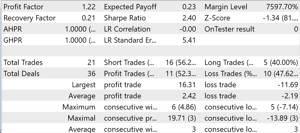
During the testing period, the model made 21 transactions, 52.3% of which were closed with a profit. Both the maximum and average profitable trades exceed the corresponding metrics for losing trades. The resulted in the profit factor of 1.22
Conclusion
In this article, we discussed an optical flow estimation method called CCMR, which combines the advantages of the concepts of context-based motion aggregation and a multi-scale coarse-to-fine approach. This produces detailed flow maps that are also highly accurate in obstructed areas.
The authors of the method proposed a two-stage motion grouping strategy in which global-context features are first calculated. These are then used to guide motion characteristics iteratively at all scales. This allows XCiT-based algorithms to process all scales from coarse to fine while preserving scale-specific content.
In the practical part of the article, we implemented the proposed approaches using MQL5. We trained and tested the model using real data in the MetaTrader 5 strategy tester. The results obtained suggest the effectiveness of the proposed approaches.
However, let me remind you that all the programs presented in the article are of an informative nature and are intended only to demonstrate the proposed approaches.
References
Programs used in the article
| # | Issued to | Type | Description |
|---|---|---|---|
| 1 | Research.mq5 | EA | Example collection EA |
| 2 | ResearchRealORL.mq5 | EA | EA for collecting examples using the Real-ORL method |
| 3 | Study.mq5 | EA | Model training EA |
| 4 | Test.mq5 | EA | Model testing EA |
| 5 | Trajectory.mqh | Class library | System state description structure |
| 6 | NeuroNet.mqh | Class library | A library of classes for creating a neural network |
| 7 | NeuroNet.cl | Code Base | OpenCL program code library |
Translated from Russian by MetaQuotes Ltd.
Original article: https://www.mql5.com/ru/articles/14505
Warning: All rights to these materials are reserved by MetaQuotes Ltd. Copying or reprinting of these materials in whole or in part is prohibited.
This article was written by a user of the site and reflects their personal views. MetaQuotes Ltd is not responsible for the accuracy of the information presented, nor for any consequences resulting from the use of the solutions, strategies or recommendations described.

- Free trading apps
- Over 8,000 signals for copying
- Economic news for exploring financial markets
You agree to website policy and terms of use