
Neural networks made easy (Part 77): Cross-Covariance Transformer (XCiT)

Introduction
Transformers show great potential in solving problems of analyzing various sequences. The Self-Attention operation which underlies transformers, provides global interactions between all tokens in the sequence. This makes it possible to evaluate interdependencies within the entire analyzed sequence. However, this comes with quadratic complexity in terms of computation time and memory usage, making it difficult to apply the algorithm to long sequences.
To solve this problem, the authors of the paper "XCiT: Cross-Covariance Image Transformers" suggested a "transposed" version of Self-Attention, which operates through feature channels rather than tokens, where interactions are based on a cross-covariance matrix between keys and queries. The result is cross-covariance attention (XCA) with linear complexity in the number of tokens, allowing for efficient processing of large data sequences. Cross-covariance image transformer (XCiT), based on XCA, combines the accuracy of conventional transformers with the scalability of convolutional architectures. That paper experimentally confirms the effectiveness and generality of XCiT. The presented experiments demonstrate excellent results on several visual benchmarks, including image classification, object detection, and instance segmentation.
1. XCiT algorithm
The authors of the method propose the Self-Attention function based on cross-covariance, which operates along the feature dimension rather than along the token dimension, as in the classical Self-Attention tokens. Using the Query, Key and Value definitions, the cross-covariance attention function is defined as:
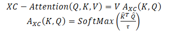
where each output token embedding is a convex combination of the dv features of its corresponding token embedding in V. The attention weights A are computed based on the cross-covariance matrix.
In addition to building a new attention function based on the cross-covariance matrix, the authors of the method propose to restrict the magnitude of the Query and Key matrices by L2-normalizing them so that each column of length N of the normalized matrices Q and K had unit norm. Every element of the cross-covariance matrix of attention coefficients of size d*d was in the range [−1, 1]. The authors of the method state that norm control significantly increases the stability of learning, especially when learning with a variable number of tokens. However, restricting the norm reduces the representational power of the operation by removing degrees of freedom. Therefore, the authors introduce a trainable temperature parameter τ which scales the inner products before performing normalization by the SoftMax function, allowing for sharper or more uniform distribution of attention weights.
In addition, the authors of the method limit the number of features that interact with each other. They propose to divide them into h groups, or "heads", similar to multi-headed Self-Attention tokens. For each head, the authors of the method separately apply cross-covariance attention.
For each head, they train separate weight matrices of source data projection X to Query, Key and Value. The corresponding weight matrices are collected in tensors Wq of dimensions {h * d * dq}, Wk — {h * d * dk} and Wv — {h * d * dv} \). They set dk = dq = dv = d/h.
Restricting attention to heads has two benefits:
- The complexity of aggregating values with attention weights is reduced by a factor h;
- more importantly, the authors of the method empirically demonstrate that the block-diagonal matrix version is easier to optimize and generally leads to improved results.
The classical Self-Attention tokens with h heads have time complexity O(N^2 * d) and memory O(hN^2 + Nd). Due to quadratic complexity, it is problematic to scale Self-Attention tokens for sequences with a large number of tokens. The proposed cross-covariance attention overcomes this drawback because its computational complexity O(Nd^2/h) scales linearly with the number of tokens. The same applies to memory complexity O(d^2 / h + Nd).
Therefore, the XCA model proposed by the authors scales much better in cases where the number of tokens N is large, and the feature dimension d is relatively small, especially when splitting the features into h heads
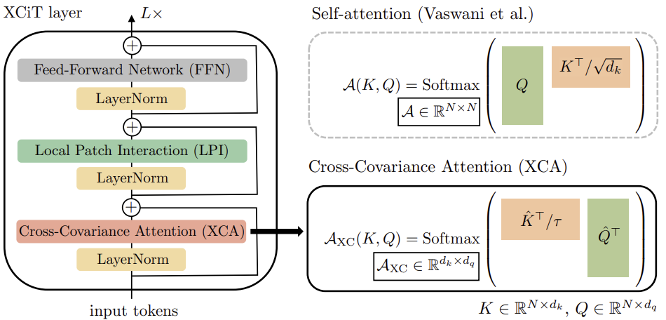
To build Cross-Covariance Transformer images (XCiT), the authors of the method propose a columnar architecture that maintains the same spatial resolution across layers. They combine the Cross-Covariance Attention block (XCA) with 2 subsequent additional modules, each of which is preceded by normalization within the layer.
In the XCA block, communication between patches is carried out only indirectly through shared statistics. To provide explicit communication between patches, the authors of the method add a simple local patch interaction block (LPI) after each XCA block. LPI consists of two convolutional layers and a batch normalization layer between them. As the activation function of the first layer, they suggest using GELU. Due to its deep block structure, LPI has negligible parameter overhead, and very limited bandwidth and memory overhead.
As is common in transformer models, a Feed-Forward Network (FFN) with pointwise convolutional layers is added next, which has one hidden layer with 4d hidden blocks. While interactions between features are limited in groups within the XCA block, and there is no interaction between the features in the LPI block, FFN allows the interaction with all features.
Unlike the attention map included in Self-Attention tokens, covariance blocks in XCiT have a fixed size, regardless of the resolution of the input sequence. SoftMax always works with the same number of elements, which may explain why XCiT models behave better when working with images of different resolutions. XCiT includes additive sine positional coding with input tokens.
The authors' visualization of the algorithm is presented below.
2. Implementation using MQL5
After considering the theoretical aspects of the Cross-Covariation Transformer (XCiT), we move on to the practical implementation of the proposed approaches using MQL5.
2.1 Cross-Covariance Transformer Class
To implement the XCiT block algorithm, we will create a new neural layer class CNeuronXCiTOCL. As the parent class, we will use the common multi-head multi-layer attention class CNeuronMLMHAttentionOCL. The new class will also be created with the built-in multi-layer architecture.
class CNeuronXCiTOCL  : public CNeuronMLMHAttentionOCL
  {
protected:
   //---
   uint              iLPIWindow;
   uint              iLPIStep;
   uint              iBatchCount;
   //---
   CCollection       cLPI;
   CCollection       cLPI_Weights;
   //---
   virtual bool      feedForward(CNeuronBaseOCL *NeuronOCL);
   virtual bool      XCiT(CBufferFloat *qkv, CBufferFloat *score, CBufferFloat *out);
   virtual bool      BatchNorm(CBufferFloat *inputs, CBufferFloat *options, CBufferFloat *out);
   //---
   virtual bool      updateInputWeights(CNeuronBaseOCL *NeuronOCL);
   virtual bool      XCiTInsideGradients(CBufferFloat *qkv, CBufferFloat *qkvg,
                                         CBufferFloat *score, CBufferFloat *aog);
   virtual bool      BatchNormInsideGradient(CBufferFloat *inputs, CBufferFloat *inputs_g,
         CBufferFloat *options, CBufferFloat *out,
         CBufferFloat *out_g, ENUM_ACTIVATION activation);
   virtual bool      BatchNormUpdateWeights(CBufferFloat *options, CBufferFloat *out_g);

public:
                     CNeuronXCiTOCL(void) {};
                    ~CNeuronXCiTOCL(void) {};
   virtual bool      Init(uint numOutputs, uint myIndex, COpenCLMy *open_cl,
                          uint window, uint lpi_window, uint heads,
                          uint units_count, uint layers,
                          ENUM_OPTIMIZATION optimization_type,
                          uint batch);
   virtual bool      calcInputGradients(CNeuronBaseOCL *prevLayer);
   //---
   virtual int       Type(void)   const   {  return defNeuronXCiTOCL;   }
   //--- methods for working with files
   virtual bool      Save(int const file_handle);
   virtual bool      Load(int const file_handle);
   virtual CLayerDescription* GetLayerInfo(void);
   virtual bool      WeightsUpdate(CNeuronBaseOCL *source, float tau);
   virtual void      SetOpenCL(COpenCLMy *obj);
  };
I would like to note that in the new class, we will make maximum use of the tools of the parent class. However, we will still need to make significant additions. First, we will add buffer collections for LPI block:
- cLPI – result and gradient buffers;
- cLPI_Weights – weight and momentum matrices.
In addition, for the LPI block we need additional constants:
- iLPIWindow – convolution window for the first layer of the block;
- iLPIStep – step of the convolution window for the first layer of the block;
- iBatchCount – the number of operations performed in the block batch normalization layer.
We specify convolution parameters only in the first layer. Since in the second layer we need to reach the size of the source data layer. Because the authors of the method propose adding and normalizing data with the results of the previous XCA block.
In this class, all added objects are declared static, so we leave the constructor and destructor of the layer empty. The primary initialization of the layer is implemented in the Init method. In parameters, the method receives all the parameters needed to initialize internal objects.
bool CNeuronXCiTOCL::Init(uint numOutputs, uint myIndex, COpenCLMy *open_cl,
                          uint window, uint lpi_window, uint heads, uint units_count,
                          uint layers, ENUM_OPTIMIZATION optimization_type, uint batch)
{
 if(!CNeuronBaseOCL::Init(numOutputs, myIndex, open_cl, window * units_count, optimization_type,
                                                                                         batch))
     return false;
In the body of the method, we do not organize a control block for the received parameters. Instead, we call the initialization method of the base class of all neural layers, which already implements the minimum necessary controls and initializes inherited objects.
The thing to note here is that we are calling the method of the base class, not the parent class. This is due to the fact that the sizes of the internal layer buffers we create, and their number will differ. Therefore, to avoid the need to perform the same work twice, we will initialize all buffers in the body of our new initialization method.
First, we save the main parameters into local variables.
   iWindow = fmax(window, 1);
   iUnits = fmax(units_count, 1);
   iHeads = fmax(fmin(heads, iWindow), 1);
   iWindowKey = fmax((window + iHeads - 1) / iHeads, 1);
   iLayers = fmax(layers, 1);
   iLPIWindow = fmax(lpi_window, 1);
   iLPIStep = 1;
Please note that we recalculate the dimensions of internal entities based on the size of the description vector of one element of the sequence and the number of attention heads. This is suggested by the authors of the XCiT method.
Next, we determine the main dimensions of the buffers in each block.
//--- XCA
   uint num = 3 * iWindowKey * iHeads * iUnits;                // Size of QKV tensor
   uint qkv_weights = 3 * (iWindow + 1) * iWindowKey * iHeads; // Size of weights' matrix of
                                                               // QKV tensor
   uint scores = iWindowKey * iWindowKey * iHeads;             // Size of Score tensor
   uint out = iWindow * iUnits;                                // Size of output tensor
//--- LPI
   uint lpi1_num = iWindow * iHeads * iUnits;                  // Size of LPI1 tensor
   uint lpi1_weights = (iLPIWindow + 1) * iHeads;              // Size of weights' matrix of
                                                               // LPI1 tensor
   uint lpi2_weights = (iHeads + 1) * 2;                       // Size of weights' matrix of
                                                               // LPI2 tensor
//--- FF
   uint ff_1 = 4 * (iWindow + 1) * iWindow;           // Size of weights' matrix 1-st
                                                      // feed forward layer
   uint ff_2 = (4 * iWindow + 1) * iWindow;           // Size of weights' matrix 2-nd
                                                      // feed forward layer
After that we organize a loop with the number of iterations equal to the number of internal layers.
   for(uint i = 0; i < iLayers; i++)
     {
      CBufferFloat *temp = NULL;
In the body of the loop, we first create buffers of intermediate results and their gradients. For this, we create a nested loop. In the first iteration of the loop, we create buffers of intermediate results. In the second iteration, we create the buffers of the corresponding error gradients.
      for(int d = 0; d < 2; d++)
        {
         //--- XCiT
         //--- Initilize QKV tensor
         temp = new CBufferFloat();
         if(CheckPointer(temp) == POINTER_INVALID)
            return false;
         if(!temp.BufferInit(num, 0))
            return false;
         if(!temp.BufferCreate(OpenCL))
            return false;
         if(!QKV_Tensors.Add(temp))
            return false;
Let's combine Query, Key and Value into one concatenated buffer. This will allow us to generate the values of all entities in one pass for all attention heads in parallel threads.
Next, we create a reduced buffer of cross-covariance attention coefficients.
         //--- Initialize scores
         temp = new CBufferFloat();
         if(CheckPointer(temp) == POINTER_INVALID)
            return false;
         if(!temp.BufferInit(scores, 0))
            return false;
         if(!temp.BufferCreate(OpenCL))
            return false;
         if(!S_Tensors.Add(temp))
            return false;
The attention block ends with its results buffer.
         //--- Initialize attention out
         temp = new CBufferFloat();
         if(CheckPointer(temp) == POINTER_INVALID)
            return false;
         if(!temp.BufferInit(out, 0))
            return false;
         if(!temp.BufferCreate(OpenCL))
            return false;
         if(!AO_Tensors.Add(temp))
            return false;
The approach proposed by the authors of the method for computing the size of entities allows us to remove the layer of reducing the dimension of the attention block.
Next we create the buffers of the LPI block. Here we create a buffer of the results of the first convolution layer.
         //--- LPI
         //--- Initilize LPI tensor
         temp = new CBufferFloat();
         if(CheckPointer(temp) == POINTER_INVALID)
            return false;
         if(!temp.BufferInit(lpi1_num, 0))
            return false;
         if(!temp.BufferCreate(OpenCL))
            return false;
         if(!cLPI.Add(temp))                             // LPI1
            return false;
This is followed by a buffer of batch normalization results.
         temp = new CBufferFloat();
         if(CheckPointer(temp) == POINTER_INVALID)
            return false;
         if(!temp.BufferInit(lpi1_num, 0))
            return false;
         if(!temp.BufferCreate(OpenCL))
            return false;
         if(!cLPI.Add(temp))                             // LPI Normalize
            return false;
The block ends with the result buffer of the second convolutional layer.
         temp = new CBufferFloat();
         if(CheckPointer(temp) == POINTER_INVALID)
            return false;
         if(!temp.BufferInit(out, 0))
            return false;
         if(!temp.BufferCreate(OpenCL))
            return false;
         if(!cLPI.Add(temp))                             // LPI2
            return false;
Finally, we create the buffers of the FeedForward block result.
         //--- Initialize Feed Forward 1
         temp = new CBufferFloat();
         if(CheckPointer(temp) == POINTER_INVALID)
            return false;
         if(!temp.BufferInit(4 * out, 0))
            return false;
         if(!temp.BufferCreate(OpenCL))
            return false;
         if(!FF_Tensors.Add(temp))
            return false;
Pay attention to the nuance with the results buffer of the second layer of the block. We create this buffer only for intermediate data. For the last inner layer, we do not create new buffers, but only save a pointer to the previously created result buffer of our layer.
         //--- Initialize Feed Forward 2
         if(i == iLayers - 1)
           {
            if(!FF_Tensors.Add(d == 0 ? Output : Gradient))
               return false;
            continue;
           }
         temp = new CBufferFloat();
         if(CheckPointer(temp) == POINTER_INVALID)
            return false;
         if(!temp.BufferInit(out, 0))
            return false;
         if(!temp.BufferCreate(OpenCL))
            return false;
         if(!FF_Tensors.Add(temp))
            return false;
        }
We will create the weight matrix buffers in the same order.
      //--- XCiT
      //--- Initialize QKV weights
      temp = new CBufferFloat();
      if(CheckPointer(temp) == POINTER_INVALID)
         return false;
      if(!temp.Reserve(qkv_weights))
         return false;
      float k = (float)(1 / sqrt(iWindow + 1));
      for(uint w = 0; w < qkv_weights; w++)
        {
         if(!temp.Add((GenerateWeight() - 0.5f)* k))
            return false;
        }
      if(!temp.BufferCreate(OpenCL))
         return false;
      if(!QKV_Weights.Add(temp))
         return false;
      //--- Initialize LPI1
      temp = new CBufferFloat();
      if(CheckPointer(temp) == POINTER_INVALID)
         return false;
      if(!temp.Reserve(lpi1_weights))
         return false;
      for(uint w = 0; w < lpi1_weights; w++)
        {
         if(!temp.Add((GenerateWeight() - 0.5f)* k))
            return false;
        }
      if(!temp.BufferCreate(OpenCL))
         return false;
      if(!cLPI_Weights.Add(temp))
         return false;
      //--- Normalization
      int count = (int)lpi1_num * (optimization_type == SGD ? 7 : 9);
      temp = new CBufferFloat();
      if(!temp.BufferInit(count, 0.0f))
         return false;
      if(!temp.BufferCreate(OpenCL))
         return false;
      if(!cLPI_Weights.Add(temp))
         return false;
      //--- Initialize LPI2
      temp = new CBufferFloat();
      if(CheckPointer(temp) == POINTER_INVALID)
         return false;
      if(!temp.Reserve(lpi2_weights))
         return false;
      for(uint w = 0; w < lpi2_weights; w++)
        {
         if(!temp.Add((GenerateWeight() - 0.5f)* k))
            return false;
        }
      if(!temp.BufferCreate(OpenCL))
         return false;
      if(!cLPI_Weights.Add(temp))
         return false;
      //--- Initialize FF Weights
      temp = new CBufferFloat();
      if(CheckPointer(temp) == POINTER_INVALID)
         return false;
      if(!temp.Reserve(ff_1))
         return false;
      for(uint w = 0; w < ff_1; w++)
        {
         if(!temp.Add((GenerateWeight() - 0.5f)* k))
            return false;
        }
      if(!temp.BufferCreate(OpenCL))
         return false;
      if(!FF_Weights.Add(temp))
         return false;
      temp = new CBufferFloat();
      if(CheckPointer(temp) == POINTER_INVALID)
         return false;
      if(!temp.Reserve(ff_2))
         return false;
      k = (float)(1 / sqrt(4 * iWindow + 1));
      for(uint w = 0; w < ff_2; w++)
        {
         if(!temp.Add((GenerateWeight() - 0.5f)* k))
            return false;
        }
      if(!temp.BufferCreate(OpenCL))
         return false;
      if(!FF_Weights.Add(temp))
         return false;
After initializing the trainable weight matrices, we create buffers to record momentums during the model training process. But here you should pay attention to the parameter buffer of the batch normalization layer. It already takes into account the parameters and their momentums. Therefore, we will not create momentum buffers for the specified layer.
In addition, the number of required momentum buffers depends on the optimization method. To take this feature into account, we will create buffers in a loop, the number of iterations of which depends on the optimization method.
      for(int d = 0; d < (optimization == SGD ? 1 : 2); d++)
        {
         //--- XCiT
         temp = new CBufferFloat();
         if(CheckPointer(temp) == POINTER_INVALID)
            return false;
         if(!temp.BufferInit(qkv_weights, 0))
            return false;
         if(!temp.BufferCreate(OpenCL))
            return false;
         if(!QKV_Weights.Add(temp))
            return false;
         //--- LPI
         temp = new CBufferFloat();
         if(CheckPointer(temp) == POINTER_INVALID)
            return false;
         if(!temp.BufferInit(lpi1_weights, 0))
            return false;
         if(!temp.BufferCreate(OpenCL))
            return false;
         if(!cLPI_Weights.Add(temp))
            return false;
         temp = new CBufferFloat();
         if(CheckPointer(temp) == POINTER_INVALID)
            return false;
         if(!temp.BufferInit(lpi2_weights, 0))
            return false;
         if(!temp.BufferCreate(OpenCL))
            return false;
         if(!cLPI_Weights.Add(temp))
            return false;
         //--- FF Weights momentus
         temp = new CBufferFloat();
         if(CheckPointer(temp) == POINTER_INVALID)
            return false;
         if(!temp.BufferInit(ff_1, 0))
            return false;
         if(!temp.BufferCreate(OpenCL))
            return false;
         if(!FF_Weights.Add(temp))
            return false;
         temp = new CBufferFloat();
         if(CheckPointer(temp) == POINTER_INVALID)
            return false;
         if(!temp.BufferInit(ff_2, 0))
            return false;
         if(!temp.BufferCreate(OpenCL))
            return false;
         if(!FF_Weights.Add(temp))
            return false;
        }
     }
   iBatchCount = 1;
//---
   return true;
  }
After successfully creating all the necessary buffers, we terminate the method and return the logical result of the operations to the caller.
We have completed the initialization of the class. Now, let's proceed to the description of the feed-forward algorithm of the XCiT method. As mentioned above, the implementation of the proposed method will require significant changes. To implement feed-forward pass, we need to create a kernel on the side of the OpenCL program to implement the XCA algorithm.
Please note that we receive the entities in a method inherited from the parent class ConvolutionForward. So, our kernel already works with the generated Query, Key and Value entities, which we transfer to the kernel as a single buffer. In addition to them, in the kernel parameters we pass pointers to two more data buffers: attention coefficients and attention block results.
__kernel void XCiTFeedForward(__global float *qkv,
                              __global float *score,
                              __global float *out)
  {
   const size_t d = get_local_id(0);
   const size_t dimension = get_local_size(0);
   const size_t u = get_local_id(1);
   const size_t units = get_local_size(1);
   const size_t h = get_global_id(2);
   const size_t heads = get_global_size(2);
We will launch the kernel in a 3-dimensional task space:
- dimension of one entity element;
- sequence length;
- number of attention heads.
As for the first two dimensions, we will combine them into local working groups.
Let's declare two local 2-dimensional arrays for writing intermediate data and exchanging information within the working group.
   const uint ls_u = min((uint)units, (uint)LOCAL_ARRAY_SIZE);
   const uint ls_d = min((uint)dimension, (uint)LOCAL_ARRAY_SIZE);
   __local float q[LOCAL_ARRAY_SIZE][LOCAL_ARRAY_SIZE];
   __local float k[LOCAL_ARRAY_SIZE][LOCAL_ARRAY_SIZE];
Before starting work on analyzing cross-covariance attention, we need to normalize the Query and Key entities, as proposed by the authors of the method.
To do this, we first compute the sizes of vectors for each parameter within the group.
//--- Normalize Query and Key
   for(int cur_d = 0; cur_d < dimension; cur_d += ls_d)
     {
      float q_val = 0;
      float k_val = 0;
      //---
      if(d < ls_d && (cur_d + d) < dimension && u < ls_u)
        {
         for(int count = u; count < units; count += ls_u)
           {
            int shift = count * dimension * heads * 3 + dimension * h + cur_d + d;
            q_val += pow(qkv[shift], 2.0f);
            k_val += pow(qkv[shift + dimension * heads], 2.0f);
           }
         q[u][d] = q_val;
         k[u][d] = k_val;
        }
      barrier(CLK_LOCAL_MEM_FENCE);
      uint count = ls_u;
      do
        {
         count = (count + 1) / 2;
         if(d < ls_d)
           {
            if(u < ls_u && u < count && (u + count) < units)
              {
               float q_val = q[u][d] + q[u + count][d];
               float k_val = k[u][d] + k[u + count][d];
               q[u + count][d] = 0;
               k[u + count][d] = 0;
               q[u][d] = q_val;
               k[u][d] = k_val;
              }
           }
         barrier(CLK_LOCAL_MEM_FENCE);
        }
      while(count > 1);
Then we divide each element in the sequence by the square root of the vector size along the corresponding dimension.
      int shift = u * dimension * heads * 3 + dimension * h + cur_d;
      qkv[shift] = qkv[shift] / sqrt(q[0][d]);
      qkv[shift + dimension * heads] = qkv[shift + dimension * heads] / sqrt(k[0][d]);
      barrier(CLK_LOCAL_MEM_FENCE);
     }
Now that our entities are normalized, we can move on to defining dependency coefficients. To do this, we multiply the Query and Key matrices. At the same time, we take the exponent of the obtained value and sum them up.
//--- Score
   int step = dimension * heads * 3;
   for(int cur_r = 0; cur_r < dimension; cur_r += ls_u)
     {
      for(int cur_d = 0; cur_d < dimension; cur_d += ls_d)
        {
         if(u < ls_d && d < ls_d)
            q[u][d] = 0;
         barrier(CLK_LOCAL_MEM_FENCE);
         //---
         if((cur_r + u) < ls_d && (cur_d + d) < ls_d)
           {
            int shift_q = dimension * h + cur_d + d;
            int shift_k = dimension * (heads + h) + cur_r + u;
            float scr = 0;
            for(int i = 0; i < units; i++)
               scr += qkv[shift_q + i * step] * qkv[shift_k + i * step];
            scr = exp(scr);
            score[(cur_r + u)*dimension * heads + dimension * h + cur_d + d] = scr;
            q[u][d] += scr;
           }
        }
      barrier(CLK_LOCAL_MEM_FENCE);
      int count = ls_d;
      do
        {
         count = (count + 1) / 2;
         if(u < ls_d)
           {
            if(d < ls_d && d < count && (d + count) < dimension)
               q[u][d] += q[u][d + count];
            if(d + count < ls_d)
               q[u][d + count] = 0;
           }
         barrier(CLK_LOCAL_MEM_FENCE);
        }
      while(count > 1);
Then we normalize the dependence coefficients.
      if((cur_r + u) < ls_d)
         score[(cur_r + u)*dimension * heads + dimension * h + d] /= q[u][0];
      barrier(CLK_LOCAL_MEM_FENCE);
     }
At the end of the kernel operations, we multiply the Value tensor by the dependence coefficients. The result of this operation will be saved in the results buffer of the XCA attention block.
   int shift_out = dimension * (u * heads + h) + d;
   int shift_s = dimension * (heads * d + h);
   int shift_v = dimension * (heads * (u * 3 + 2) + h);
   float sum = 0;
   for(int i = 0; i < dimension; i++)
      sum += qkv[shift_v + i] * score[shift_s + i];
   out[shift_out] = sum;
  }
After creating the kernel on the OpenCL program side, we move on to operations in our class on the side of the main program. Here we first create the CNeuronXCiTOCL::XCiT method, in which we implement the algorithm for calling the created kernel.
bool CNeuronXCiTOCL::XCiT(CBufferFloat *qkv, CBufferFloat *score, CBufferFloat *out)
  {
   if(!OpenCL || !qkv || !score || !out)
      return false;
In the method parameters, we pass pointers to the 3 used data buffers. In the method body, we immediately check if the received pointers are relevant.
Then we define the task space and the offsets in it.
   uint global_work_offset[3] = {0, 0, 0};
   uint global_work_size[3] = {iWindowKey, iUnits, iHeads};
   uint local_work_size[3] = {iWindowKey, iUnits, 1};
As mentioned above, we combine threads into working groups along the first two dimensions.
Next, we pass pointers to data buffers to the kernel.
   if(!OpenCL.SetArgumentBuffer(def_k_XCiTFeedForward, def_k_XCiTff_qkv, qkv.GetIndex()))
      return false;
   if(!OpenCL.SetArgumentBuffer(def_k_XCiTFeedForward, def_k_XCiTff_score, score.GetIndex()))
      return false;
   if(!OpenCL.SetArgumentBuffer(def_k_XCiTFeedForward, def_k_XCiTff_out, out.GetIndex()))
      return false;
Put the kernel in the execution queue.
   ResetLastError();
   if(!OpenCL.Execute(def_k_XCiTFeedForward, 3, global_work_offset, global_work_size,
                                                                    local_work_size))
     {
      printf("Error of execution kernel %s: %d", __FUNCTION__, GetLastError());
      string error;
      CLGetInfoString(OpenCL.GetContext(), CL_ERROR_DESCRIPTION, error);
      Print(error);
      return false;
     }
//---
   return true;
  }
In addition to the method described above, we will create a feed-forward method for the batch normalization layer CNeuronXCiTOCL::BatchNorm, the entire algorithm of which is fully transferred from the CNeuronBatchNormOCL::feedForward method. But we will not dwell now on considering its algorithm. Let's move directly to the analysis of the CNeuronXCiTOCL::feedForward method, which represents the general outline of the forward propagation algorithm in the XCiT block.
bool CNeuronXCiTOCL::feedForward(CNeuronBaseOCL *NeuronOCL)
  {
   if(CheckPointer(NeuronOCL) == POINTER_INVALID)
      return false;
In the parameters, the method receives a pointer to the object of the previous layer, which provides the initial data. In the method body, we immediately check the relevance of the received pointer.
After successfully passing the control point, we create a loop through the internal layers. In the body of this loop, we will construct the entire algorithm of the method.
   for(uint i = 0; (i < iLayers && !IsStopped()); i++)
     {
      //--- Calculate Queries, Keys, Values
      CBufferFloat *inputs = (i == 0 ? NeuronOCL.getOutput() : FF_Tensors.At(4 * i - 2));
      CBufferFloat *qkv = QKV_Tensors.At(i * 2);
      if(IsStopped() || !ConvolutionForward(QKV_Weights.At(i * (optimization == SGD ? 2 : 3)),
                                           inputs, qkv, iWindow, 3 * iWindowKey * iHeads, None))
         return false;
Here we first form our Query, Key and Value entities. Then we call our cross-covariance attention method.
      //--- Score calculation
      CBufferFloat *temp = S_Tensors.At(i * 2);
      CBufferFloat *out = AO_Tensors.At(i * 2);
      if(IsStopped() || !XCiT(qkv, temp, out))
         return false;
The attention results are added to the original data and the resulting values are normalized.
      //--- Sum and normalize attention
      if(IsStopped() || !SumAndNormilize(out, inputs, out, iWindow, true))
         return false;
Next comes the LPI block. First, let's organize the work of the first layer of the block.
      //--- LPI
      inputs = out;
      temp = cLPI.At(i * 6);
      if(IsStopped() || !ConvolutionForward(cLPI_Weights.At(i * (optimization == SGD ? 5 : 7)),
                                            inputs, temp, iLPIWindow, iHeads, LReLU, iLPIStep))
         return false;
Then we normalize the results of the first layer.
      out = cLPI.At(i * 6 + 1);
      if(IsStopped() || !BatchNorm(temp, cLPI_Weights.At(i * (optimization == SGD ? 5 : 7) + 1),
                                                                                           out))
         return false;
We pass the normalized result to the second layer of the block.
    temp = out;
    out = cLPI.At(i * 6 + 2);
    if(IsStopped() ||!ConvolutionForward(cLPI_Weights.At(i * (optimization == SGD ? 5 : 7) + 2),
                                                        temp, out, 2 * iHeads, 2, None, iHeads))
       return false;
Then we summarize and normalize the results again.
      //--- Sum and normalize attention
      if(IsStopped() || !SumAndNormilize(out, inputs, out, iWindow, true))
         return false;
Organize the FeedForward block.
     //--- Feed Forward
     inputs = out;
     temp = FF_Tensors.At(i * 4);
     if(IsStopped() || !ConvolutionForward(FF_Weights.At(i * (optimization == SGD ? 4 : 6)),
                                                 inputs, temp, iWindow, 4 * iWindow, LReLU))
        return false;
     out = FF_Tensors.At(i * 4 + 1);
     if(IsStopped() || !ConvolutionForward(FF_Weights.At(i * (optimization == SGD ? 4 : 6) + 1),
                                                   temp, out, 4 * iWindow, iWindow, activation))
        return false;
At the output of the layer, we summarize and normalize the results of the blocks.
      //--- Sum and normalize out
      if(IsStopped() || !SumAndNormilize(out, inputs, out, iWindow, true))
         return false;
     }
   iBatchCount++;
//---
   return true;
  }
This concludes the implementation of the feed-forward pass of our new Cross-Covariance transformer layer CNeuronXCiTOCL. Next, we move on to constructing the backpropagation algorithm. Here we also have to return to the OpenCL program and create another kernel. We will build the backpropagation algorithm of the XCA block in the XCiTInsideGradients kernel. In the parameters to the kernel, we pass pointers to 4 data buffers:
- qkv – concatenated vector of Query, Key and Value entities;
- qkv_g – concatenated vector of error gradients of Query, Key and Value entities;
- scores – matrix of dependence coefficients;
- gradient – tensor of error gradients at the output of the XCA attention block.
__kernel void XCiTInsideGradients(__global float *qkv, __global float *qkv_g,
                                  __global float *scores,
                                  __global float *gradient)
  {
//--- init
   const int q = get_global_id(0);
   const int d = get_global_id(1);
   const int h = get_global_id(2);
   const int units = get_global_size(0);
   const int dimension = get_global_size(1);
   const int heads = get_global_size(2);
We plan to launch the kernel in a 3-dimensional task space. In the body of the kernel, we identify the thread and task space. Then we determine the offset in the data buffers to the analyzed elements.
   const int shift_q = dimension * (heads * 3 * q + h);
   const int shift_k = dimension * (heads * (3 * q + 1) + h);
   const int shift_v = dimension * (heads * (3 * q + 2) + h);
   const int shift_g = dimension * (heads * q + h);
   int shift_score = dimension * h;
   int step_score = dimension * heads;
According to the backpropagation algorithm, we first determine the error gradient on the Value tensor.
//--- Calculating Value's gradients
   float sum = 0;
   for(int i = 0; i < dimension; i ++)
      sum += gradient[shift_g + i] * scores[shift_score + d + i * step_score];
   qkv_g[shift_v + d] = sum;
Next, we define the error gradient for Query. Here we have to first determine the error gradient on the corresponding vector of the coefficient matrix. Then adjust the resulting error gradients to the derivative of the SoftMax function. Only in this case can we obtain the required error gradient.
//--- Calculating Query's gradients
   float grad = 0;
   float val = qkv[shift_v + d];
   for(int k = 0; k < dimension; k++)
     {
      float sc_g = 0;
      float sc = scores[shift_score + k];
      for(int v = 0; v < dimension; v++)
         sc_g += scores[shift_score + v] * val * gradient[shift_g + v * dimension] *
                                                              ((float)(k == v) - sc);
      grad += sc_g * qkv[shift_k + k];
     }
   qkv_g[shift_q] = grad;
For the Key tensor, the error gradient is determined similarly, but in the perpendicular direction of the vectors.
//--- Calculating Key's gradients
   grad = 0;
   float out_g = gradient[shift_g];
   for(int scr = 0; scr < dimension; scr++)
     {
      float sc_g = 0;
      int shift_sc = scr * dimension * heads;
      float sc = scores[shift_sc + d];
      for(int v = 0; v < dimension; v++)
         sc_g += scores[shift_sc + v] * out_g * qkv[shift_v + v] * ((float)(d == v) - sc);
      grad += sc_g * qkv[shift_q + scr];
     }
   qkv_g[shift_k + d] = grad;
  }
After building the kernel, we return to working with our class on the side of the main program. Here we create the CNeuronXCiTOCL::XCiTInsideGradients method. In the parameters, the method receives pointers to the required data buffers.
bool CNeuronXCiTOCL::XCiTInsideGradients(CBufferFloat *qkv, CBufferFloat *qkvg,
                                         CBufferFloat *score, CBufferFloat *aog)
  {
   if(!OpenCL || !qkv || !qkvg || !score || !aog)
      return false;
In the method body, we immediately check if the received pointers are relevant.
Then we define a 3-dimensional problem space. But this time we don't define workgroups.
   uint global_work_offset[3] = {0, 0, 0};
   uint global_work_size[3] = {iWindowKey, iUnits, iHeads};
We pass pointers to data buffers as parameters to the kernel.
   if(!OpenCL.SetArgumentBuffer(def_k_XCiTInsideGradients, def_k_XCiTig_qkv, qkv.GetIndex()))
      return false;
   if(!OpenCL.SetArgumentBuffer(def_k_XCiTInsideGradients, def_k_XCiTig_qkv_g, qkvg.GetIndex()))
      return false;
   if(!OpenCL.SetArgumentBuffer(def_k_XCiTInsideGradients, def_k_XCiTig_scores,score.GetIndex()))
      return false;
   if(!OpenCL.SetArgumentBuffer(def_k_XCiTInsideGradients, def_k_XCiTig_gradient,aog.GetIndex()))
      return false;
After completing the preparatory work, we only need to put the kernel in the execution queue.
   ResetLastError();
   if(!OpenCL.Execute(def_k_XCiTInsideGradients, 3, global_work_offset, global_work_size))
     {
      printf("Error of execution kernel %s: %d", __FUNCTION__, GetLastError());
      return false;
     }
//---
   return true;
  }
The complete backward algorithm of the XCiT block collected in the dispatch method CNeuronXCiTOCL::calcInputGradients. In its parameters, the method receives a pointer to the object of the previous layer.
bool CNeuronXCiTOCL::calcInputGradients(CNeuronBaseOCL *prevLayer)
  {
   if(CheckPointer(prevLayer) == POINTER_INVALID)
      return false;
In the body of the method, we immediately check the validity of the received pointer. After successfully passing the control point, we organize a loop of the reverse iteration through the internal layers with the propagation of the error gradient.
   CBufferFloat *out_grad = Gradient;
//---
   for(int i = int(iLayers - 1); (i >= 0 && !IsStopped()); i--)
     {
      //--- Passing gradient through feed forward layers
      if(IsStopped() || !ConvolutionInputGradients(FF_Weights.At(i*(optimization==SGD ? 4:6)+1),
                                                   out_grad, FF_Tensors.At(i * 4),
                                                   FF_Tensors.At(i * 4 + 2), 4 * iWindow,
                                                   iWindow, None))
         return false;
In the body of the loop, we will first pass the error gradient through the FeedForward block.
      CBufferFloat *temp = cLPI.At(i * 6 + 5);
      if(IsStopped() ||
         !ConvolutionInputGradients(FF_Weights.At(i * (optimization == SGD ? 4 : 6)),
                                    FF_Tensors.At(i * 4 + 1), cLPI.At(i * 6 + 2), temp,
                                    iWindow, 4 * iWindow, LReLU))
         return false;
Let me remind you that during the direct pass, we added the results of the blocks with the original data. Similarly, we propagate the error gradient across 2 threads.
      //--- Sum and normalize gradients
      if(IsStopped() || !SumAndNormilize(out_grad, temp, temp, iWindow, false))
         return false;
Next we propagate the error gradient through the LPI block.
      out_grad = temp;
      //--- Passing gradient through LPI
      if(IsStopped() ||
         !ConvolutionInputGradients(cLPI_Weights.At(i * (optimization == SGD ? 5 : 7) + 2),
                                    temp, cLPI.At(i * 6 + 1), cLPI.At(i * 6 + 4),

                                    2 * iHeads, 2, None, 0, iHeads))
         return false;
      if(IsStopped() ||
         !BatchNormInsideGradient(cLPI.At(i * 6), cLPI.At(i * 6 + 3),
                                  cLPI_Weights.At(i * (optimization == SGD ? 5 : 7) + 1),
                                  cLPI.At(i * 6 + 1),  cLPI.At(i * 6 + 4), LReLU))
         return false;
      if(IsStopped() ||
         !ConvolutionInputGradients(cLPI_Weights.At(i * (optimization == SGD ? 5 : 7)),
                                    cLPI.At(i * 6 + 3), AO_Tensors.At(i * 2),
                                    AO_Tensors.At(i * 2 + 1),  iLPIWindow, iHeads,
                                    None, 0, iLPIStep))
         return false;
Add the error gradients again.
      temp = AO_Tensors.At(i * 2 + 1);
      //--- Sum and normalize gradients
      if(IsStopped() || !SumAndNormilize(out_grad, temp, temp, iWindow, false))
         return false;
After that, we propagate the error gradient through the attention block XCA.
      out_grad = temp;
      //--- Passing gradient to query, key and value
      if(IsStopped() ||
         !XCiTInsideGradients(QKV_Tensors.At(i * 2), QKV_Tensors.At(i * 2 + 1),
                              S_Tensors.At(i * 2), temp))
         return false;
Transfer it to the source data gradient buffer.
      CBufferFloat *inp = NULL;
      if(i == 0)
        {
         inp = prevLayer.getOutput();
         temp = prevLayer.getGradient();
        }
      else
        {
         temp = FF_Tensors.At(i * 4 - 1);
         inp = FF_Tensors.At(i * 4 - 3);
        }
      if(IsStopped() ||
         !ConvolutionInputGradients(QKV_Weights.At(i * (optimization == SGD ? 2 : 3)),
                                    QKV_Tensors.At(i * 2 + 1), inp, temp, iWindow,
                                    3 * iWindowKey * iHeads, None))
         return false;
Don't forget to add an error gradient along the second stream.
      //--- Sum and normalize gradients
      if(IsStopped() || !SumAndNormilize(out_grad, temp, temp, iWindow))
         return false;
      if(i > 0)
         out_grad = temp;
     }
//---
   return true;
  }
Above, we implemented an algorithm for propagating the error gradient to the internal layers and transferring it to the previous neural layer. At the end of the backpropagation operations, we need to update the model parameters.
Updating the parameters of our new Cross-Covariance Transformer layer is implemented in the CNeuronXCiTOCL::updateInputWeights method. Like similar methods of other neural layers, the method receives a pointer to the neural layer of the previous layer in its parameters.
bool CNeuronXCiTOCL::updateInputWeights(CNeuronBaseOCL *NeuronOCL)
  {
   if(CheckPointer(NeuronOCL) == POINTER_INVALID)
      return false;
   CBufferFloat *inputs = NeuronOCL.getOutput();
And in the body of the method, we check the relevance of the received pointer.
Similar to the distribution of the error gradient, we will update the parameters in a loop through the inner layers.
   for(uint l = 0; l < iLayers; l++)
     {
      if(IsStopped() ||
         !ConvolutuionUpdateWeights(QKV_Weights.At(l * (optimization == SGD ? 2 : 3)),
                                    QKV_Tensors.At(l * 2 + 1), inputs,
                                   (optimization==SGD ? QKV_Weights.At(l*2+1):QKV_Weights.At(l*3+1)),
                                   (optimization==SGD ? NULL : QKV_Weights.At(l*3+2)),
                                    iWindow, 3 * iWindowKey * iHeads))
         return false;
First, we update the parameters of the formation matrices for the Query, Key and Value entities.
Next, we update the parameters of the LPI block. This block contains 2 convolutional layers and a batch normalization layer.
      if(IsStopped() ||
         !ConvolutuionUpdateWeights(cLPI_Weights.At(l * (optimization == SGD ? 5 : 7)),
                                    cLPI.At(l * 6 + 3), AO_Tensors.At(l * 2),
                                   (optimization==SGD ? cLPI_Weights.At(l*5+3):cLPI_Weights.At(l*7+3)),
                                   (optimization==SGD ? NULL : cLPI_Weights.At(l * 7 + 5)),
                                    iLPIWindow, iHeads, iLPIStep))
         return false;
      if(IsStopped() ||
         !BatchNormUpdateWeights(cLPI_Weights.At(l * (optimization == SGD ? 5 : 7) + 1),
                                 cLPI.At(l * 6 + 4)))
         return false;
      if(IsStopped() ||
         !ConvolutuionUpdateWeights(cLPI_Weights.At(l * (optimization == SGD ? 5 : 7) + 2),
                                    cLPI.At(l * 6 + 5), cLPI.At(l * 6 + 1),
                                   (optimization==SGD ? cLPI_Weights.At(l*5+4):cLPI_Weights.At(l*7+4)),
                                   (optimization==SGD ? NULL : cLPI_Weights.At(l * 7 + 6)),
                                    2 * iHeads, 2, iHeads))
         return false;
At the end of the method, we have the block that updates the parameters of the FeedForward block.
      if(IsStopped() ||
         !ConvolutuionUpdateWeights(FF_Weights.At(l * (optimization == SGD ? 4 : 6)),
                                    FF_Tensors.At(l * 4 + 2), cLPI.At(l * 6 + 2),
                                   (optimization==SGD ? FF_Weights.At(l*4+2):FF_Weights.At(l*6+2)),
                                   (optimization==SGD ? NULL : FF_Weights.At(l * 6 + 4)),
                                   iWindow, 4 * iWindow))
         return false;
      //---
      if(IsStopped() ||
         !ConvolutuionUpdateWeights(FF_Weights.At(l * (optimization == SGD ? 4 : 6) + 1),
                                    FF_Tensors.At(l * 4 + 3), FF_Tensors.At(l * 4),
                                   (optimization==SGD ? FF_Weights.At(l*4+3):FF_Weights.At(l*6+3)),
                                   (optimization==SGD ? NULL : FF_Weights.At(l * 6 + 5)),
                                    4 * iWindow, iWindow))
         return false;
      inputs = FF_Tensors.At(l * 4 + 1);
     }
//---
   return true;
  }
With this we complete the implementation of the feed-forward and backpropagation algorithms of our Cross-Covariance transformer layer CNeuronXCiTOCL. To enable the full operation of the class, we still need to add several auxiliary methods. Among them are File methods (Save and Load). The algorithm of these methods is not complicated and does not contain any unique aspects which relate specifically to the XCiT method. Therefore, I will not dwell on the description of their algorithms in this article. The attachment contains the full code of the class, so you can study it yourself. The attachment also contains all programs used in this article.
2.2 Model architecture
We move on to building Expert Advisors for training and testing the models. It must be said here that in their paper, the authors of the method did not present a specific architecture of the models. Essentially, the proposed Cross-Covariance Transformer can replace the classical Transformer we considered earlier in any model. Therefore, as part of the experiment, we can take the model from the previous articles and replace the CNeuronMLMHAttentionOCL layer with CNeuronXCiTOCL.
But we have to be honest here. In the previous article, we used different blocks of attention. We especially focused on using CNeuronMFTOCL, which, due to its architectural features, cannot be replaced with CNeuronXCiTOCL.
However, replacing even one layer allows us to somehow evaluate the changes.
So, the final architecture of our test model is as follows.
bool CreateTrajNetDescriptions(CArrayObj *encoder, CArrayObj *endpoints, CArrayObj *probability)
  {
//---
   CLayerDescription *descr;
//---
   if(!encoder)
     {
      encoder = new CArrayObj();
      if(!encoder)
         return false;
     }
   if(!endpoints)
     {
      endpoints = new CArrayObj();
      if(!endpoints)
         return false;
     }
   if(!probability)
     {
      probability = new CArrayObj();
      if(!probability)
         return false;
     }
"Raw" source data describing 1 bar is fed to the source data layer of the environmental encoder.
//--- Encoder
   encoder.Clear();
//--- Input layer
   if(!(descr = new CLayerDescription()))
      return false;
   descr.type = defNeuronBaseOCL;
   int prev_count = descr.count = (HistoryBars * BarDescr);
   descr.activation = None;
   descr.optimization = ADAM;
   if(!encoder.Add(descr))
     {
      delete descr;
      return false;
     }
The received data is processed in the batch normalization layer.
//--- layer 1
   if(!(descr = new CLayerDescription()))
      return false;
   descr.type = defNeuronBatchNormOCL;
   descr.count = prev_count;
   descr.batch = MathMax(1000, GPTBars);
   descr.activation = None;
   descr.optimization = ADAM;
   if(!encoder.Add(descr))
     {
      delete descr;
      return false;
     }
An environmental state embedding is generated from the normalized data and added to the internal stack.
//--- layer 2
   if(!(descr = new CLayerDescription()))
      return false;
   descr.type = defNeuronEmbeddingOCL;
     {
      int temp[] = {prev_count};
      ArrayCopy(descr.windows, temp);
     }
   prev_count = descr.count = GPTBars;
   int prev_wout = descr.window_out = EmbeddingSize;
   if(!encoder.Add(descr))
     {
      delete descr;
      return false;
     }
Here we also add positional data encoding.
//--- layer 3
   if(!(descr = new CLayerDescription()))
      return false;
   descr.type = defNeuronPEOCL;
   descr.count = prev_count;
   descr.window = prev_wout;
   if(!encoder.Add(descr))
     {
      delete descr;
      return false;
     }
This is followed by a graph block with batch normalization between layers.
//--- layer 4
   if(!(descr = new CLayerDescription()))
      return false;
   descr.type = defNeuronCGConvOCL;
   descr.count = prev_count * prev_wout;
   descr.window = descr.count;
   if(!encoder.Add(descr))
     {
      delete descr;
      return false;
     }
//--- layer 5
   if(!(descr = new CLayerDescription()))
      return false;
   descr.type = defNeuronBatchNormOCL;
   descr.count = prev_count * prev_wout;
   descr.batch = MathMax(1000, GPTBars);
   descr.activation = None;
   descr.optimization = ADAM;
   if(!encoder.Add(descr))
     {
      delete descr;
      return false;
     }
//--- layer 6
   if(!(descr = new CLayerDescription()))
      return false;
   descr.type = defNeuronCGConvOCL;
   descr.count = prev_count * prev_wout;
   descr.window = descr.count;
   if(!encoder.Add(descr))
     {
      delete descr;
      return false;
     }
Next, we add our new Cross-Covariation Transformer layer. We left the number of sequence elements and source data windows unchanged. The specified parameters are determined by the tensor of the initial data.
//--- layer 7
   if(!(descr = new CLayerDescription()))
      return false;
   descr.type = defNeuronXCiTOCL;
   descr.count = prev_count;
   descr.window = prev_wout;
   descr.step = 4;
   descr.window_out = 3;
   descr.layers = 1;
   descr.batch = MathMax(1000, GPTBars);
   descr.optimization = ADAM;
   if(!encoder.Add(descr))
     {
      delete descr;
      return false;
     }
In this case, we use 4 attention heads.
The authors of the method propose to use an integer splitting of the size of the description vector of one sequence element to determine the size of the entity vector per the number of attention heads. With this option, our descr.window_out parameter is not used. So, let's take advantage of this fact and specify the size of the window of the first LPI layer in this parameter. We also indicate the batch size to normalize the data in the LPI block.
The encoder is followed by the MFT block.
//--- layer 8
   if(!(descr = new CLayerDescription()))
      return false;
   descr.type = defNeuronMFTOCL;
   descr.count = prev_count;
   descr.window = prev_wout;
   descr.step = 4;
   descr.window_out = 16;
   descr.layers = NForecast;
   descr.optimization = ADAM;
   if(!encoder.Add(descr))
     {
      delete descr;
      return false;
     }
We transpose the tensor to convert it into the appropriate form.
//--- layer 9
   if(!(descr = new CLayerDescription()))
      return false;
   descr.type = defNeuronTransposeOCL;
   descr.count = prev_count;
   descr.window = prev_wout * NForecast;
   if(!encoder.Add(descr))
     {
      delete descr;
      return false;
     }
The results of the environmental encoder and MFT are used to decode the most likely endpoints.
//--- Endpoints
   endpoints.Clear();
//--- Input layer
   if(!(descr = new CLayerDescription()))
      return false;
   descr.type = defNeuronBaseOCL;
   descr.count = (prev_count * prev_wout) * NForecast;
   descr.activation = None;
   descr.optimization = ADAM;
   if(!endpoints.Add(descr))
     {
      delete descr;
      return false;
     }
//--- layer 1
   if(!(descr = new CLayerDescription()))
      return false;
   descr.type = defNeuronConvOCL;
   descr.count = NForecast * prev_wout;
   descr.window = prev_count;
   descr.step = descr.window;
   descr.window_out = LatentCount;
   descr.activation = SIGMOID;
   descr.optimization = ADAM;
   if(!endpoints.Add(descr))
     {
      delete descr;
      return false;
     }
//--- layer 2
   if(!(descr = new CLayerDescription()))
      return false;
   descr.type = defNeuronConvOCL;
   descr.count = NForecast;
   descr.window = LatentCount * prev_wout;
   descr.step = descr.window;
   descr.window_out = 3;
   descr.activation = None;
   descr.optimization = ADAM;
   if(!endpoints.Add(descr))
     {
      delete descr;
      return false;
     }
And their probability estimates.
//--- Probability
   probability.Clear();
//--- Input layer
   if(!probability.Add(endpoints.At(0)))
      return false;
//--- layer 1
   if(!(descr = new CLayerDescription()))
      return false;
   descr.type = defNeuronConcatenate;
   descr.count = LatentCount;
   descr.window = prev_count * prev_wout * NForecast;
   descr.step = 3 * NForecast;
   descr.optimization = ADAM;
   descr.activation = SIGMOID;
   if(!probability.Add(descr))
     {
      delete descr;
      return false;
     }
//--- layer 2
   if(!(descr = new CLayerDescription()))
      return false;
   descr.type = defNeuronBaseOCL;
   descr.count = LatentCount;
   descr.activation = LReLU;
   descr.optimization = ADAM;
   if(!probability.Add(descr))
     {
      delete descr;
      return false;
     }
//--- layer 3
   if(!(descr = new CLayerDescription()))
      return false;
   descr.type = defNeuronBaseOCL;
   descr.count = NForecast;
   descr.activation = None;
   descr.optimization = ADAM;
   if(!probability.Add(descr))
     {
      delete descr;
      return false;
     }
//--- layer 4
   if(!(descr = new CLayerDescription()))
      return false;
   descr.type = defNeuronSoftMaxOCL;
   descr.count = NForecast;
   descr.step = 1;
   descr.activation = None;
   descr.optimization = ADAM;
   if(!probability.Add(descr))
     {
      delete descr;
      return false;
     }
//---
   return true;
  }
The Actor model did not use attention layers. Therefore, the model was copied without changes. And you can familiarize yourself with the complete architecture of all models in the attachment.
Note that replacing one layer in the architecture of the environmental state encoder does not affect the organization of the model training and testing processes. Therefore, all training and environmental interaction EAs have been copied without changes. In my opinion, this way it is more interesting to view testing results. Because keeping other things equal, we can most honestly assess the impact of replacing a layer in the model architecture.
And you can find the complete code of all programs used herein in the attachment. We move on to testing the constructed Cross-Covariance Transformer layer CNeuronXCiTOCL.
3. Testing
We have done quite substantial work to build a new Cross-Covariance Transformer class CNeuronXCiTOCL based on the algorithm presented in the paper "XCiT: Cross-Covariance Image Transformers". As mentioned above, we have decided to use the Expert Advisor from the previous article in an unchanged form. Therefore, to train the models, we can use the previously collected training dataset. Let's just rename the file "MFT.bd" to "XCiT.bd".
If you do not have a previously collected training dataset, then you need to collect it before training the model. I recommend first collecting data from real signals using the method described in the article "Using past experience to solve new problems". Then you should supplement the training dataset with random passes of the EA "...\Experts\XCiT\Research.mq5" in the strategy tester.
The models are trained in the EA "...\Experts\XCiT\Study.mq5" after collecting the training data.
As before, the model is trained on EURUSD H1 historical data. All indicators are used with default parameters.
The model is trained on historical data for the first 7 months of 2023. Here we can immediately note the first results of testing the effectiveness of the proposed approaches. During the training process, we can see a reduction in time costs of almost 2% while having the same training iterations.
The effectiveness of the trained model was assessed using historical data for August 2023. The testing period is not included in the training dataset. However, it comes directly after the training period. Based on the results of testing the trained model, we got the results close to those presented in the previous article.
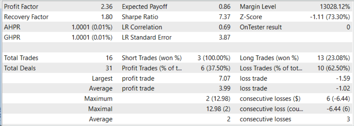
However, behind a slight increase in the number of trades there is an increase in the profit factor.
Conclusion
In this article, we got acquainted with the new architecture of the Cross-Covariance Transformer (XCiT), which combines the advantages of Transformers and Convolutional architectures. It provides high accuracy and scalability when processing sequences of varying lengths. Some efficiency is achieved when analyzing large sequences with small token sizes.
XCiT uses a Cross-Covariance Attention architecture to efficiently model global interactions between features of sequence elements, allowing it to successfully handle long sequences of tokens.
The authors of the method experimentally confirm its high efficiency of XCiT on several visual tasks, including image classification, object detection, and semantic segmentation.
In the practical part of our article, we implemented the proposed methods using MQL5. The model was trained and tested on real historical data. During the training process, we had a slight reduction in training time for the same number of trained iterations. This was achieved by replacing only one layer in the model.
A slight increase in the efficiency of the trained model may indicate a better generalization ability of the proposed architecture.
Please don't forget that trading in financial markets is a high-risk investment. All programs presented in the article are provided for informational purposes only and are not optimized for real trading.
References
Programs used in the article
| # | Issued to | Type | Description |
|---|---|---|---|
| 1 | Research.mq5 | Expert Advisor | EA for collecting examples |
| 2 | ResearchRealORL.mq5 | Expert Advisor | EA for collecting examples using the Real-ORL method |
| 3 | Study.mq5 | Expert Advisor | Model training EA |
| 4 | Test.mq5 | Expert Advisor | Model testing EA |
| 5 | Trajectory.mqh | Class library | System state description structure |
| 6 | NeuroNet.mqh | Class library | A library of classes for creating a neural network |
| 7 | NeuroNet.cl | Code Base | OpenCL program code library |
Translated from Russian by MetaQuotes Ltd.
Original article: https://www.mql5.com/ru/articles/14276
Warning: All rights to these materials are reserved by MetaQuotes Ltd. Copying or reprinting of these materials in whole or in part is prohibited.
This article was written by a user of the site and reflects their personal views. MetaQuotes Ltd is not responsible for the accuracy of the information presented, nor for any consequences resulting from the use of the solutions, strategies or recommendations described.

- Free trading apps
- Over 8,000 signals for copying
- Economic news for exploring financial markets
You agree to website policy and terms of use