
Neural networks made easy (Part 76): Exploring diverse interaction patterns with Multi-future Transformer

Introduction
Predicting upcoming price movements is one of the key prerequisites to building a successful trading strategy. Therefore, we need to explore the possibilities of creating accurate and multimodal forecasts of future movement. In previous articles, we got acquainted with some methods for predicting price movements. Among them were multimodal ones, offering several event development variants.
However, they all rarely focus on future possibilities of interaction between the analyzed agents, which can lead to loss of information and suboptimal forecasting. In addition, it is quite difficult to scale previously discussed methods in case we have multiple agents, since independent predictions can lead to an exponential number of combinations. Most of the resulting combinations are not feasible due to conflicting predictions. Therefore, it is important to focus on predicting scenes as a whole, estimating the future state of multiple agents simultaneously.
The authors of the paper "Multi-future Transformer: Learning diverse interaction modes for behavior prediction in autonomous driving" suggest using the Multi-future Transformer (MFT) method to solve such problems. Its main idea is to decompose the multimodal distribution of the future into several unimodal distributions, which allows you to effectively simulate various models of interaction between agents on the scene.
In MFT, forecasts are generated by a neural network with fixed parameters in a single feed-forward pass, without the need to stochastically sample latent variables, pre-determine anchors, or run an iterative post-processing algorithm. This allows the model to operate in a deterministic, repeatable manner.
1. Multi-future Transformer algorithm
The main goal of the Multi-future Transformer method is to consistently predict future movement Y of all the agents in the scene. To do this, it analyzes the dynamic state of agents X and the contextual information M. Thus, the overall probability distribution to capture is P(Y|X,M), which is multimodal as a result of the clear evolution of the scene.
It is usually very difficult to directly model joint multimodal distribution. The authors of the method introduce the assumption that the target distribution can be decomposed into a mixture of several unimodal distributions, and then these unimodal distributions are modeled separately, which is formulated as
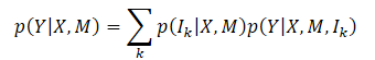
where Ik represents the k-th mode component;
p(Ik|X,M) is the probability distribution of different modes;
p(Y|X,M,Ik) represents the factorized unimodal distribution.
Under this formulation, the key point in MFT is that the main difference between each target distribution mode lies in the different interaction models between agents, and between agents and context. Modeling of each unimodal distribution can be realized by studying the patterns of mode-correspondence interactions. Intuitively, future scene uncertainty can be mainly decomposed into two parts: intention uncertainty and interaction uncertainty.
Unobservable intentions can be well captured by modeling the interaction between the agent and the context, since the endpoint of the future trajectory, representing the agent's intentions, is closely related to the context of the scene. To account for the uncertainty of interaction, different modes of interaction between agents are modeled. Thus, by jointly capturing agent-to-agent interactions as well as agent-to-context interactions, future uncertainty is minimized and the evolution of a scene can be determined.
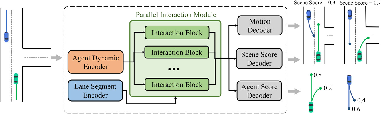
To achieve the multimodal joint distribution decomposition described above, the general architecture of the proposed MFT approach was designed. It consists of three parts:
- Encoders
- Parallel interaction module
- Prediction headers
The model includes two types of encoders:
- The dynamic agent encoder is used to extract features from observed dynamic states,
- The context segment encoder serves as a map viewer to learn pointwise functions for stripe points.
The core of the MFT model is a parallel interaction module, which consists of several interaction blocks in a parallel structure and studies the future features of the movement of agents for each mode. The three prediction headers include:
- Motion decoder,
- Agent score decoder,
- Scene score decoder.
They are responsible for decoding future trajectories for each agent and estimating confidence scores for each predicted trajectory and each scene mode. In this architecture, the paths along which the feed-forward and backpropagation signals of each mode pass are independent of each other, and each path contains a unique interaction block that provides information interaction between signals of the same mode. Therefore, interaction units can simultaneously capture the corresponding interaction patterns of different modes. However, encoders and prediction headers are common to each mode, while interaction blocks are parameterized as different objects. Therefore, each unimodal distribution, which theoretically has different parameters, can be modeled in a more parameter-efficient way. The original visualization of the method is shown below.
The observed trajectories of agents on the historical horizon can be represented as X={x1,...,xatt}, where the dynamic state at each time step xt=(x,y,vx,vy,w) contains position (x,y), velocity (vx,vy), and yaw angle w at that time.
The dynamic states of an agent are considered as a set of points in a multidimensional space, where each point is represented by coordinates (x,y), and other dimensions represent additional local features. For these points, the interaction properties and the given local structure are preserved, since the observed states of the agent interact with each other and together form the agent's observed trajectory. In addition, another important property of these trajectory points is the temporal order, which is an implicit features compared to static lane points. Naturally, the same trajectory points with a reverse time order lead to a completely different observed trajectory. The above properties require the model to represent trajectory points not only by combining point features, but also by introducing temporal order information. For this purpose, absolute positional encoding is used to encode ordering information. The model calculates dynamic features for each agent as follows:
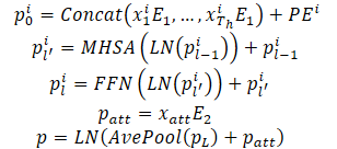
Multiple encoder layers are stacked to improve the model's ability to represent dynamic information. Averaging is performed over all points of an agent's trajectory to summarize historical dynamic information related to a specific agent.
Point features corresponding to the current moment were also extracted to obtain dynamic information. This provides performance similar to the average pool. When dealing with partially observable historical states, a Self-Attention-based framework can simply mask out unobservable positions without additional effort, thereby effectively avoiding feature confusion caused by invalid padding.
A distinctive characteristic of the behavior prediction task is the multimodality caused by future scene uncertainty. A common approach is to use multiple result headers to independently decode each agent's future trajectories based on a common feature vector. However, this method has two main disadvantages:
- The motion information of various possible future trajectories is contained in one feature vector with a fixed dimension, which leads to limited information and significantly limits the expressive capabilities of the model;
- The forward and backward signals from different modes are mixed through feature interaction and gradient propagation, leading to the mode confusion problem that degrades the ability to make multimodal predictions.
Instead, in MFT, interaction modeling is divided into different modes to achieve a multimodal outcome by learning the unique interaction pattern corresponding to each mode. For this purpose, a parallel interaction module was designed. This module contains several blocks of parallel interaction, each of which represents a certain mode of future development of events. In this structure, intra-mode forward and backward signals cross the interaction block of the corresponding mode. At the same time, other modes do not interfere, which avoids the problem of mode confusion.
In addition, each interaction block is parameterized as a separate object, allowing the model to have sufficient expressive power to cope with the large variation between different modes. Each interaction block uses a Self-Attention mechanism to model the interaction between agents and the Cross-Attention mechanism to capture the interaction between agents and the scene. These two types of interaction features are added to the dynamic feature through residual connection to obtain the final upcoming motion function for each agent and mode. The above process can be described as follows:

The final structure of the parallel interaction module can be seen as parallelizing the Transformer decoder with a serial structure. However, multimodal prediction and increased expressive power are achieved at similar computational cost compared to its standard counterpart. Experiments conducted by the authors of the method confirm that, in combination with the use of the winner-take-all loss strategy at the scene level, the proposed method can provide consistent prediction of the behavior of several agents. A study was also conducted to demonstrate the indispensability of the two types of modeled interactions and the reasonability of the module structure design.
The authors' visualization of the module structure is presented below.

In addition to predicting the future trajectory of each agent, MFT runs a likelihood estimation for each possible development of the scene, as well as for each predicted trajectory of the agent. For motion planning tasks, the ideal input would be a multimodal scene prediction with an appropriate confidence score for each scene mode. The planning algorithm can directly calculate the possible future motion trajectory by considering all neighboring agents simultaneously. For this purpose, the authors of the method developed heads for predicting various scenes and their probabilities.
To estimate the probability at the scene level, the feature vectors of all agents in the scene are averaged. This allows us to get a scene-level view.
In addition, to pay special attention to the agent, the likelihood estimation should be performed from the viewpoint of the agent itself. Consequently, a third model header is created to decode confidence estimates of each agent's predicted trajectories. The Multi-future Transformer decoding process is formulated as follows:
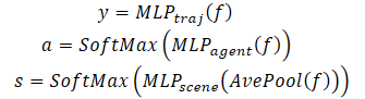
Note that to decode a multimodal scene, a decoder with the same parameters is used for all possible scenarios.
2. Implementation using MQL5
After considering the theoretical aspects of the Multi-future Transformer method, let us move on to the practical part of our article. Let us consider how to implement the algorithm in MQL5.
From the above description of the Multi-future Transformer algorithm, we can say that the main implementation difficulty for us is the parallel interaction module. Our library already has previously implemented multi-head Self-Attention (CNeuronMLMHAttentionOCL) and Cross-Attention (CNeuronMH2AttentionOCL) layers. However, even when using several heads of attention, the data flows in them are mixed during forward and backward passes. This does not satisfy the conditions of the Multi-future Transformer method.
Therefore, we will begin our implementation of the method by creating a class of a new neural layer.
2.1. Parallel interaction module
We implement the parallel interaction module algorithm in the CNeuronMFTOCL class, which we inherit from CNeuronMLMHAttentionOCL.
This class was chosen as the parent on purpose. CNeuronMLMHAttentionOCL already contains an implemented functionality of the multi-layer Self-Attention algorithm. We use the existing code in implementing the new class. But instead of sequentially computing the layers of the attention block, we will predict various scenarios. In addition, we will add Cross-Attention functionality provided by the Multi-future Transformer algorithm.
The structure of the new class is shown below. As you can see, in addition to redefining the main methods, we are adding another collection of data buffers for data transposition, which we will need in order to implement the Cross-Attention mechanism.
class CNeuronMFTOCL  : public CNeuronMLMHAttentionOCL
  {
protected:
   //---
   CCollection       cTranspose;
   //---
   virtual bool      feedForward(CNeuronBaseOCL *NeuronOCL);
   virtual bool      Transpose(CBufferFloat *in, CBufferFloat *out, int rows, int cols);
   virtual bool      MHCA(CBufferFloat *q, CBufferFloat *kv,
                          CBufferFloat *score, CBufferFloat *out);
   //---
   virtual bool      updateInputWeights(CNeuronBaseOCL *NeuronOCL);
   virtual bool      MHCAInsideGradients(CBufferFloat *q, CBufferFloat *qg,
                                         CBufferFloat *kv, CBufferFloat *kvg,
                                         CBufferFloat *score, CBufferFloat *aog);

public:
                     CNeuronMFTOCL(void) {};
                    ~CNeuronMFTOCL(void) {};
   virtual bool      Init(uint numOutputs, uint myIndex, COpenCLMy *open_cl,
                          uint window, uint window_key, uint heads,
                          uint units_count, uint features,
                          ENUM_OPTIMIZATION optimization_type,
                          uint batch);
   virtual bool      calcInputGradients(CNeuronBaseOCL *prevLayer);
   //---
   virtual int       Type(void)   const   {  return defNeuronMFTOCL;   }
   //--- methods for working with files
   virtual bool      Save(int const file_handle);
   virtual bool      Load(int const file_handle);
   virtual CLayerDescription* GetLayerInfo(void);
   virtual bool      WeightsUpdate(CNeuronBaseOCL *source, float tau);
   virtual void      SetOpenCL(COpenCLMy *obj);
  };
Declaring a new collection of data buffers as static allows us to leave the constructor and destructor of the class "empty". We initialize the class and internal objects in the Init method.
bool CNeuronMFTOCL::Init(uint numOutputs, uint myIndex, COpenCLMy *open_cl,
                         uint window, uint window_key, uint heads, uint units_count,
                         uint features, ENUM_OPTIMIZATION optimization_type, uint batch)
  {
   if(!CNeuronBaseOCL::Init(numOutputs, myIndex, open_cl, window * units_count * features,
                                                                optimization_type, batch))
      return false;
In the parameters, the method receives all the necessary information to recreate the required architecture. In the body of the method, we call the relevant method of the neural layer base class CNeuronBaseOCL.
Please note that we are not calling the initialization method of the direct parent class CNeuronMLMHAttentionOCL. Instead, we turn higher – to the base class of neural layers CNeuronBaseOCL. This is due to some differences in the implementation of CNeuronMFTOCL and CNeuronMLMHAttentionOCL.
In the CNeuronMLMHAttentionOCL parent class we sequentially processed the source data in several layers of the attention block and at the output we received a result with a dimension similar to the source data. Now in the new CNeuronMFTOCL layer, we will consistently generate various patterns for possible developments. Accordingly, the result of the layer will be a multiple (by the number of forecast options) of the size of the original data. Therefore, we need to increase the results buffer.
In addition, to avoid unnecessary copying of data, in the parent class we replaced the buffer of results and gradients of the layer itself and of the last internal layer. In implementing the new class, this approach is unacceptable, since we have to concatenate the results of several parallel blocks into a single buffer.
Let's get back to our initialization method. After successfully executing the neural layer base class initialization method, we save the key parameters of the architecture into internal class variables.
   iWindow = fmax(window, 1);
   iWindowKey = fmax(window_key, 1);
   iUnits = fmax(units_count, 1);
   iHeads = fmax(heads, 1);
   iLayers = fmax(features, 1);
Please note that we save all parameters in variables of the parent class. Here we have a slight deviation between the name of the variable and its functionality: the iLayers variable will store the number of planned options. In order to use resources more efficiently, I decided not to create an additional variable and "ignore" the discrepancy between the name and functionality of the variable.
Next, we will calculate the main parameters of our blocks.
//--- MHSA
   uint num = 3 * iWindowKey * iHeads * iUnits;       //Size of QKV tensor
   uint qkv_weights = 3 * (iWindow + 1) * iWindowKey * iHeads;
                                                      //Size of weights' matrix of QKV tensor
   uint scores = iUnits * iUnits * iHeads;            //Size of Score tensor
   uint mh_out = iWindowKey * iHeads * iUnits;        //Size of multi-heads self-attention
   uint out = iWindow * iUnits;                       //Size of output tensor
   uint w0 = (iWindowKey + 1) * iHeads * iWindow;     //Size W0 tensor
//--- MHCA
   uint num_q = iWindowKey * iHeads * iUnits;         //Size of Q tensor
   uint num_kv = 2 * iWindowKey * iHeads * iUnits;    //Size of KV tensor
   uint q_weights = (iWindow + 1) * iWindowKey * iHeads;
                                                      //Size of weights' matrix of Q tensor
   uint kv_weights = 2 * (iUnits + 1) * iWindowKey * iHeads;
                                                      //Size of weights' matrix of KV tensor
   uint scores_ca = iUnits * iWindow * iHeads;            //Size of Score tensor
//--- FF
   uint ff_1 = 4 * (iWindow + 1) * iWindow;    //Size of weights' matrix 1-st feed forward layer
   uint ff_2 = (4 * iWindow + 1) * iWindow;    //Size of weights' matrix 2-nd feed forward layer
After completing the preparatory work, we will organize a loop in which we will sequentially create data buffers for each scenario in our parallel interaction block.
   for(uint i = 0; i < iLayers; i++)
     {
      CBufferFloat *temp = NULL;
      for(int d = 0; d < 2; d++)
        {
         //--- MHSA
         //--- Initilize QKV tensor
         temp = new CBufferFloat();
         if(CheckPointer(temp) == POINTER_INVALID)
            return false;
         if(!temp.BufferInit(num, 0))
            return false;
         if(!temp.BufferCreate(OpenCL))
            return false;
         if(!QKV_Tensors.Add(temp))
            return false;
Here we will create a nested loop to create forward and backward pass buffers. In the body of the nested loop, we first create a buffer of concatenated Query, Key and Value embeddings of the MHSA block. We also add a buffer for the 'Score' matrix.
         //--- Initialize scores
         temp = new CBufferFloat();
         if(CheckPointer(temp) == POINTER_INVALID)
            return false;
         if(!temp.BufferInit(scores, 0))
            return false;
         if(!temp.BufferCreate(OpenCL))
            return false;
         if(!S_Tensors.Add(temp))
            return false;
Add a buffer of multi-headed attention results.
         //--- Initialize multi-heads attention out
         temp = new CBufferFloat();
         if(CheckPointer(temp) == POINTER_INVALID)
            return false;
         if(!temp.BufferInit(mh_out, 0))
            return false;
         if(!temp.BufferCreate(OpenCL))
            return false;
         if(!AO_Tensors.Add(temp))
            return false;
At the output of the MHSA block, we create a buffer for combining the results of different attention heads.
         //--- Initialize attention out
         temp = new CBufferFloat();
         if(CheckPointer(temp) == POINTER_INVALID)
            return false;
         if(!temp.BufferInit(out, 0))
            return false;
         if(!temp.BufferCreate(OpenCL))
            return false;
         if(!FF_Tensors.Add(temp))
            return false;
It should be noted here that to satisfy the requirements of the MFT algorithm, the results of attention heads are combined only within one interaction mode.
Next we create similar buffers for the Cross-Attention block (MHCA). However, now we separate the Query embedding buffer from Key and Value, since different source data will be used.
         //--- MHCA
         //--- Initilize QKV tensor
         temp = new CBufferFloat();
         if(CheckPointer(temp) == POINTER_INVALID)
            return false;
         if(!temp.BufferInit(num_q, 0))
            return false;
         if(!temp.BufferCreate(OpenCL))
            return false;
         if(!QKV_Tensors.Add(temp))
            return false;
         temp = new CBufferFloat();
         if(CheckPointer(temp) == POINTER_INVALID)
            return false;
         if(!temp.BufferInit(out, 0))
            return false;
         if(!temp.BufferCreate(OpenCL))
            return false;
         if(!cTranspose.Add(temp))
            return false;
         temp = new CBufferFloat();
         if(CheckPointer(temp) == POINTER_INVALID)
            return false;
         if(!temp.BufferInit(num_kv, 0))
            return false;
         if(!temp.BufferCreate(OpenCL))
            return false;
         if(!QKV_Tensors.Add(temp))
            return false;
         //--- Initialize scores
         temp = new CBufferFloat();
         if(CheckPointer(temp) == POINTER_INVALID)
            return false;
         if(!temp.BufferInit(scores_ca, 0))
            return false;
         if(!temp.BufferCreate(OpenCL))
            return false;
         if(!S_Tensors.Add(temp))
            return false;
         //--- Initialize multi-heads cross attention out
         temp = new CBufferFloat();
         if(CheckPointer(temp) == POINTER_INVALID)
            return false;
         if(!temp.BufferInit(mh_out, 0))
            return false;
         if(!temp.BufferCreate(OpenCL))
            return false;
         if(!AO_Tensors.Add(temp))
            return false;
         //--- Initialize attention out
         temp = new CBufferFloat();
         if(CheckPointer(temp) == POINTER_INVALID)
            return false;
         if(!temp.BufferInit(out, 0))
            return false;
         if(!temp.BufferCreate(OpenCL))
            return false;
         if(!FF_Tensors.Add(temp))
            return false;
After creating the buffers for the attention blocks, we create the FeedForward block buffers.
         //--- Initialize Feed Forward 1
         temp = new CBufferFloat();
         if(CheckPointer(temp) == POINTER_INVALID)
            return false;
         if(!temp.BufferInit(4 * out, 0))
            return false;
         if(!temp.BufferCreate(OpenCL))
            return false;
         if(!FF_Tensors.Add(temp))
            return false;
         //--- Initialize Feed Forward 2
         temp = new CBufferFloat();
         if(CheckPointer(temp) == POINTER_INVALID)
            return false;
         if(!temp.BufferInit(out, 0))
            return false;
         if(!temp.BufferCreate(OpenCL))
            return false;
         if(!FF_Tensors.Add(temp))
            return false;
        }
We have created buffers of the results and error gradients of individual blocks. Next, we need to create matrices of trainable weights for these blocks. We create them in the same sequence. First, we generate weights for Query, Key and Value embeddings of the MHSA block.
      //--- MHSA
      //--- Initilize QKV weights
      temp = new CBufferFloat();
      if(CheckPointer(temp) == POINTER_INVALID)
         return false;
      if(!temp.Reserve(qkv_weights))
         return false;
      float k = (float)(1 / sqrt(iWindow + 1));
      for(uint w = 0; w < qkv_weights; w++)
        {
         if(!temp.Add((GenerateWeight() - 0.5f)* k))
            return false;
        }
      if(!temp.BufferCreate(OpenCL))
         return false;
      if(!QKV_Weights.Add(temp))
         return false;
And a layer for combining attention heads.
      //--- Initilize Weights0
      temp = new CBufferFloat();
      if(CheckPointer(temp) == POINTER_INVALID)
         return false;
      if(!temp.Reserve(w0))
         return false;
      for(uint w = 0; w < w0; w++)
        {
         if(!temp.Add((GenerateWeight() - 0.5f)* k))
            return false;
        }
      if(!temp.BufferCreate(OpenCL))
         return false;
      if(!FF_Weights.Add(temp))
         return false;
Repeat operations for the MHCA block.
      //--- MHCA
      //--- Initilize Q weights
      temp = new CBufferFloat();
      if(CheckPointer(temp) == POINTER_INVALID)
         return false;
      if(!temp.Reserve(q_weights))
         return false;
      for(uint w = 0; w < q_weights; w++)
        {
         if(!temp.Add((GenerateWeight() - 0.5f)* k))
            return false;
        }
      if(!temp.BufferCreate(OpenCL))
         return false;
      if(!QKV_Weights.Add(temp))
         return false;
      //--- Initilize KV weights
      temp = new CBufferFloat();
      if(CheckPointer(temp) == POINTER_INVALID)
         return false;
      if(!temp.Reserve(kv_weights))
         return false;
      float kv = (float)(1 / sqrt(iUnits + 1));
      for(uint w = 0; w < kv_weights; w++)
        {
         if(!temp.Add((GenerateWeight() - 0.5f)* kv))
            return false;
        }
      if(!temp.BufferCreate(OpenCL))
         return false;
      if(!QKV_Weights.Add(temp))
         return false;
      //--- Initilize Weights0
      temp = new CBufferFloat();
      if(CheckPointer(temp) == POINTER_INVALID)
         return false;
      if(!temp.Reserve(w0))
         return false;
      for(uint w = 0; w < w0; w++)
        {
         if(!temp.Add((GenerateWeight() - 0.5f)* k))
            return false;
        }
      if(!temp.BufferCreate(OpenCL))
         return false;
      if(!FF_Weights.Add(temp))
         return false;
Create matrices for the FeedForward block.
      //--- Initilize FF Weights
      temp = new CBufferFloat();
      if(CheckPointer(temp) == POINTER_INVALID)
         return false;
      if(!temp.Reserve(ff_1))
         return false;
      for(uint w = 0; w < ff_1; w++)
        {
         if(!temp.Add((GenerateWeight() - 0.5f)* k))
            return false;
        }
      if(!temp.BufferCreate(OpenCL))
         return false;
      if(!FF_Weights.Add(temp))
         return false;
      //---
      temp = new CBufferFloat();
      if(CheckPointer(temp) == POINTER_INVALID)
         return false;
      if(!temp.Reserve(ff_2))
         return false;
      k = (float)(1 / sqrt(4 * iWindow + 1));
      for(uint w = 0; w < ff_2; w++)
        {
         if(!temp.Add((GenerateWeight() - 0.5f)* k))
            return false;
        }
      if(!temp.BufferCreate(OpenCL))
         return false;
      if(!FF_Weights.Add(temp))
         return false;
After that we implement another nested loop, in which we create buffers for updating the weight matrices. Note that the number of moment buffers depends on the chosen optimization algorithm.
      for(int d = 0; d < (optimization == SGD ? 1 : 2); d++)
        {
         //--- MHSA
         temp = new CBufferFloat();
         if(CheckPointer(temp) == POINTER_INVALID)
            return false;
         if(!temp.BufferInit(qkv_weights, 0))
            return false;
         if(!temp.BufferCreate(OpenCL))
            return false;
         if(!QKV_Weights.Add(temp))
            return false;
         temp = new CBufferFloat();
         if(CheckPointer(temp) == POINTER_INVALID)
            return false;
         if(!temp.BufferInit(w0, 0))
            return false;
         if(!temp.BufferCreate(OpenCL))
            return false;
         if(!FF_Weights.Add(temp))
            return false;
         //--- MHCA
         temp = new CBufferFloat();
         if(CheckPointer(temp) == POINTER_INVALID)
            return false;
         if(!temp.BufferInit(q_weights, 0))
            return false;
         if(!temp.BufferCreate(OpenCL))
            return false;
         if(!QKV_Weights.Add(temp))
            return false;
         temp = new CBufferFloat();
         if(CheckPointer(temp) == POINTER_INVALID)
            return false;
         if(!temp.BufferInit(kv_weights, 0))
            return false;
         if(!temp.BufferCreate(OpenCL))
            return false;
         if(!QKV_Weights.Add(temp))
            return false;
         temp = new CBufferFloat();
         if(CheckPointer(temp) == POINTER_INVALID)
            return false;
         if(!temp.BufferInit(w0, 0))
            return false;
         if(!temp.BufferCreate(OpenCL))
            return false;
         if(!FF_Weights.Add(temp))
            return false;
         //--- FF Weights momentus
         temp = new CBufferFloat();
         if(CheckPointer(temp) == POINTER_INVALID)
            return false;
         if(!temp.BufferInit(ff_1, 0))
            return false;
         if(!temp.BufferCreate(OpenCL))
            return false;
         if(!FF_Weights.Add(temp))
            return false;
         temp = new CBufferFloat();
         if(CheckPointer(temp) == POINTER_INVALID)
            return false;
         if(!temp.BufferInit(ff_2, 0))
            return false;
         if(!temp.BufferCreate(OpenCL))
            return false;
         if(!FF_Weights.Add(temp))
            return false;
        }
     }
//---
   return true;
  }
After successfully initializing all the necessary data buffers, we exit the method with the true result.
We have created a lot of buffers. In order not to get confused, let's create a data buffer navigation table.
| id | QKV_Tensors | S_Tensors, AO_Tensors | FF_Tensors | QKV_Weights | FF_Weights |
|---|---|---|---|---|---|
| 0 | Query, Key, Value MHSA | MHSA | MHSA Out | Query, Key, Value MHSA | MHSA W0 |
| 1 | Query MHCA | MHCA | MHCA Out | Query MHCA | MHCA W0 |
| 2 | Key, Value MHCA | Gradient MHSA | FF1 | Key, Value MHCA | FF1 |
| 3 | Gradient Query, Key, Value MHSA | Gradient MHCA | FF2 | Momentum1 Query, Key, Value MHSA | FF2 |
| 4 | Gradient Query MHCA | Gradient MHSA Out | Momentum1 Query MHCA | Momentum1 MHSA W0 | |
| 5 | Gradient Key, Value MHCA | Gradient MHCA Out | Momentum1 Key, Value MHCA | Momentum1 MHCA W0 | |
| 6 | Gradient FF1 | Momentum2 Query, Key, Value MHSA | Momentum1 FF1 | ||
| 7 | Gradient FF2 | Momentum2 Query MHCA | Momentum1 FF2 | ||
| 8 | Momentum2 Key, Value MHCA | Momentum2 MHSA W0 | |||
| 9 | Momentum2 MHCA W0 | ||||
| 10 | Momentum2 FF1 | ||||
| 11 | Momentum2 FF2 |
After CNeuronMFTOCL class initialization, we move on to constructing a feed-forward algorithm. When implementing the MFT algorithm, we did not create new kernels on the OpenCL program side. However, to call the previously created kernels, we had to create some methods on the side of the main program. In particular, for our CNeuronMFTOCL class, we created a matrix transpose method. The method algorithm is similar to the feed-forward pas of the transpose layer. However, there are differences in details. In the parameters, the new method receives pointers to 2 data buffers (source data and results), as well as the sizes of the original matrix.
bool CNeuronMFTOCL::Transpose(CBufferFloat *in, CBufferFloat *out, int rows, int cols)
  {
   if(!in || !out)
      return false;
//---
   uint global_work_offset[2] = {0, 0};
   uint global_work_size[2] = {rows, cols};
   if(!OpenCL.SetArgumentBuffer(def_k_Transpose, def_k_tr_matrix_in, in.GetIndex()))
      return false;
   if(!OpenCL.SetArgumentBuffer(def_k_Transpose, def_k_tr_matrix_out, out.GetIndex()))
      return false;
   if(!OpenCL.Execute(def_k_Transpose, 2, global_work_offset, global_work_size))
     {
      string error;
      CLGetInfoString(OpenCL.GetContext(), CL_ERROR_DESCRIPTION, error);
      printf("%s %d Error of execution kernel Transpose: %d -> %s",
                                       __FUNCTION__, __LINE__, GetLastError(), error);
      return false;
     }
//---
   return true;
  }
Accordingly, in the body of the method, we check the received pointers to data buffers and indicate the values from the parameters in the task space dimension. The kernel calling algorithm itself remained unchanged.
The situation with the MHCA feed forward method is similar. In the method parameters we receive pointers to data buffers. The CNeuronMH2AttentionOCL::attentionOut method did not have parameters and used internal objects in its functionality.
bool CNeuronMFTOCL::MHCA(CBufferFloat *q, CBufferFloat *kv,
                         CBufferFloat *score, CBufferFloat *out)
  {
   if(!q || !kv || !score || !out)
      return false;
In the body of the method, we create the dimensions of the task space.
   uint global_work_offset[3] = {0};
   uint global_work_size[3] = {iUnits, iWindow, iHeads};
   uint local_work_size[3] = {1, iWindow, 1};
We pass the parameters to the kernel.
   ResetLastError();
   if(!OpenCL.SetArgumentBuffer(def_k_MH2AttentionOut, def_k_mh2ao_q, q.GetIndex()))
     {
      printf("Error of set parameter kernel %s: %d; line %d",
                                             __FUNCTION__, GetLastError(), __LINE__);
      return false;
     }
   if(!OpenCL.SetArgumentBuffer(def_k_MH2AttentionOut, def_k_mh2ao_kv, kv.GetIndex()))
     {
      printf("Error of set parameter kernel %s: %d; line %d",
                                             __FUNCTION__, GetLastError(), __LINE__);
      return false;
     }
   if(!OpenCL.SetArgumentBuffer(def_k_MH2AttentionOut, def_k_mh2ao_score, score.GetIndex()))
     {
      printf("Error of set parameter kernel %s: %d; line %d",
                                             __FUNCTION__, GetLastError(), __LINE__);
      return false;
     }
   if(!OpenCL.SetArgumentBuffer(def_k_MH2AttentionOut, def_k_mh2ao_out, out.GetIndex()))
     {
      printf("Error of set parameter kernel %s: %d; line %d",
                                             __FUNCTION__, GetLastError(), __LINE__);
      return false;
     }
   if(!OpenCL.SetArgument(def_k_MH2AttentionOut, def_k_mh2ao_dimension, (int)iWindowKey))
     {
      printf("Error of set parameter kernel %s: %d; line %d",
                                             __FUNCTION__, GetLastError(), __LINE__);
      return false;
     }
Add it to the queue.
   if(!OpenCL.Execute(def_k_MH2AttentionOut, 3, global_work_offset, global_work_size,
                                                                    local_work_size))
     {
      printf("Error of execution kernel %s: %d", __FUNCTION__, GetLastError());
      return false;
     }
//---
   return true;
  }
The MFT feed forward algorithm is implemented in the CNeuronMFTOCL::feedForward method. Like similar methods of other neural layers, the method receives a pointer to the previous neural layer in its parameters. In the method body, we immediately check the relevance of the received pointer.
bool CNeuronMFTOCL::feedForward(CNeuronBaseOCL *NeuronOCL)
  {
   if(CheckPointer(NeuronOCL) == POINTER_INVALID)
      return false;
Next, we organize a loop of sequential calculation of various modes for interaction between agents.
  for(uint i = 0; (i < iLayers && !IsStopped()); i++)
     {
      //--- MHSA
      //--- Calculate Queries, Keys, Values
      CBufferFloat *inputs = NeuronOCL.getOutput();
      CBufferFloat *qkv = QKV_Tensors.At(i * 6);
      if(IsStopped() || !ConvolutionForward(QKV_Weights.At(i * (optimization == SGD ? 6 : 9)),
                                           inputs, qkv, iWindow, 3 * iWindowKey * iHeads, None))
         return false;
Here we first get the Query, Key and Value entities of the MHSA block. Then we define the matrix of attention coefficients.
      //--- Score calculation
      CBufferFloat *temp = S_Tensors.At(i * 4);
      if(IsStopped() || !AttentionScore(qkv, temp, false))
         return false;
Generate the result of many-headed self-attention.
      //--- Multi-heads attention calculation
      CBufferFloat *out = AO_Tensors.At(i * 4);
      if(IsStopped() || !AttentionOut(qkv, temp, out))
         return false;
We reduce the result of multi-headed attention to the size of the original data. Let me remind you that the attention heads are combined within the framework of one variant of agent interaction.
      //--- Attention out calculation
      temp = FF_Tensors.At(i * 8);
      if(IsStopped() || !ConvolutionForward(FF_Weights.At(i * (optimization == SGD ? 8 : 12)),

                                               out, temp, iWindowKey * iHeads, iWindow, None))
         return false;
We sum the resulting tensor with the original data and normalize the operation result.
      //--- Sum and normalize attention
      if(IsStopped() || !SumAndNormilize(temp, inputs, temp, iWindow))
         return false;
Next comes the cross-attention block. Here we first define the Query entity.
      //--- MHCA
      inputs = temp;
      CBufferFloat *q = QKV_Tensors.At(i * 6 + 1);
      if(IsStopped() ||
         !ConvolutionForward(QKV_Weights.At(i * (optimization == SGD ? 6 : 9) + 1),
                             inputs, q, iWindow, iWindowKey * iHeads, None))
         return false;
Then we transpose the original data and compute the Key and Value entities.
      CBufferFloat *tr = cTranspose.At(i * 2);
      if(IsStopped() || !Transpose(inputs, tr, iUnits, iWindow))
         return false;
      CBufferFloat *kv = QKV_Tensors.At(i * 6 + 2);
      if(IsStopped() ||
         !ConvolutionForward(QKV_Weights.At(i * (optimization == SGD ? 6 : 9) + 2),
                             tr, kv, iUnits, 2 * iWindowKey * iHeads, None))
         return false;
Determine the results of multi-headed cross-attention.
      //--- Multi-heads cross attention calculation
      temp = S_Tensors.At(i * 4 + 1);
      out = AO_Tensors.At(i * 4 + 1);
      if(IsStopped() || !MHCA(q, kv, temp, out))
         return false;
The obtained results are compressed to the size of the original data.
      //--- Cross Attention out calculation
      temp = FF_Tensors.At(i * 8 + 1);
      if(IsStopped() ||
         !ConvolutionForward(FF_Weights.At(i * (optimization == SGD ? 8 : 12) + 1),
                             out, temp, iWindowKey * iHeads, iWindow, None))
         return false;
Add this to the results of the MHSA block and normalize the data.
      //--- Sum and normalize attention
      if(IsStopped() || !SumAndNormilize(temp, inputs, temp, iWindow))
         return false;
Then we organize data propagation through the FeedForward block.
      //--- Feed Forward
      inputs = temp;
      temp = FF_Tensors.At(i * 8 + 2);
      if(IsStopped() ||
         !ConvolutionForward(FF_Weights.At(i * (optimization == SGD ? 8 : 12) + 2),
                             inputs, temp, iWindow, 4 * iWindow, LReLU))
         return false;
      out = FF_Tensors.At(i * 8 + 3);
      if(IsStopped() ||
         !ConvolutionForward(FF_Weights.At(i * (optimization == SGD ? 8 : 12) + 3),
                                           temp, out, 4 * iWindow, iWindow, activation))
         return false;
FeedForward block operation results are added to the MHCA results. The received data is normalized and written to the results buffer with an offset corresponding to the analyzed interaction mode.
      //--- Sum and normalize out
      if(IsStopped() ||
         !SumAndNormilize(out, inputs, Output, iWindow, true, 0, 0, i * inputs.Total()))
         return false;
     }
//---
   return true;
  }
Next, we move on to the next iteration loop to analyze the next mode of interaction between agents on the scene.
After successfully analyzing all modes for interaction between agents, we complete the method with the result true.
During the feed-forward pass, we perform the basic functionality of analyzing the modes for the interaction of agents on the scene and predicting possible variants for further events. So, model training is not possible without implementing backpropagation methods. During the backpropagation pass the model parameters are optimized to obtain better results. Therefore, after implementing the feed-forward methods, we move on to constructing the backpropagation algorithm.
As with the feed-forward pass, to implement the backpropagation pass we will need to create an additional method MHCAInsideGradients. Its algorithm is almost completely similar to the algorithm of CNeuronMH2AttentionOCL::AttentionInsideGradients. The only difference is that MHCAInsideGradients works not with internal class objects, but with buffers received in method parameters. We have already seen the examples of such modifications earlier in this article. So, we will not dwell on a detailed consideration of the method now. You can find its full code in the attachment.
The backpropagation pass algorithm is implemented in the calcInputGradients method. In the parameters, the methos receives a pointer to the object of the previous neural layer.
bool CNeuronMFTOCL::calcInputGradients(CNeuronBaseOCL *prevLayer)
  {
   if(CheckPointer(prevLayer) == POINTER_INVALID)
      return false;
In the body of the method, we immediately check the validity of the received pointer. After that we save pointers to buffers in local variables, with which all parallel interaction blocks will work.
   CBufferFloat *out_grad = Gradient;
   CBufferFloat *inp = prevLayer.getOutput();
   CBufferFloat *grad = prevLayer.getGradient();
After finishing the preparatory work, we organize a loop to propagate error gradients through separate blocks of parallel interaction.
   for(int i = 0; (i < (int)iLayers && !IsStopped()); i++)
     {
      //--- Passing gradient through feed forward layers
      if(IsStopped() ||
         !ConvolutionInputGradients(FF_Weights.At(i * (optimization == SGD ? 8 : 12) + 3),
                                   Gradient, FF_Tensors.At(i * 8 + 2), FF_Tensors.At(i * 8 + 6),
                                    4 * iWindow, iWindow, None, i * inp.Total()))
         return false;
Here we first propagate the error gradient through the FeedForward block.
      CBufferFloat *temp = FF_Tensors.At(i * 8 + 5);
      if(IsStopped() ||
         !ConvolutionInputGradients(FF_Weights.At(i * (optimization == SGD ? 8 : 12) + 2),
                                    FF_Tensors.At(i * 8 + 6), FF_Tensors.At(i * 8 + 1),
                                    temp, iWindow, 4 * iWindow, LReLU))
         return false;
In the feed-forward pass, the results of the FeedForward block operation were added to the output of the MHCA block. Similarly, we propagate the error gradient in the opposite direction. However, this time we do not perform normalization.
      //--- Sum gradient
      if(IsStopped() ||
         !SumAndNormilize(Gradient, temp, temp, iWindow, false, i * inp.Total(), 0, 0))
         return false;
      out_grad = temp;
Next, we need to propagate the error gradient through the cross-attention module. Here, we first propagate the error gradient across the attention heads.
      //--- MHCA
      //--- Split gradient to multi-heads
      if(IsStopped() ||
         !ConvolutionInputGradients(FF_Weights.At(i * (optimization == SGD ? 8 : 12) + 1),
                                                  out_grad, AO_Tensors.At(i * 4 + 1),
                                                  AO_Tensors.At(i * 4 + 3),
                                                  iWindowKey * iHeads, iWindow, None))
         return false;
Then we propagate the error gradient to the corresponding entities.
      if(IsStopped() ||
         !MHCAInsideGradients(QKV_Tensors.At(i * 6 + 1), QKV_Tensors.At(i * 6 + 4),
                              QKV_Tensors.At(i * 6 + 2), QKV_Tensors.At(i * 6 + 5),
                              S_Tensors.At(i * 4 + 1), AO_Tensors.At(i * 4 + 3)))
         return false;
Now we need to transpose the error gradient from Key and Value of the MHCA block.
      CBufferFloat *tr = cTranspose.At(i * 2 + 1);
      if(IsStopped() || !Transpose(QKV_Tensors.At(i * 6 + 5), tr, iWindow, iUnits))
         return false;
We first sum up the results obtained.
      //--- Sum
      temp = FF_Tensors.At(i * 8 + 4);
      if(IsStopped() || !SumAndNormilize(QKV_Tensors.At(i * 6 + 4), tr, temp, iWindow, false))
         return false;
Then we add to them the error gradient at the output of the MHCA block.
      if(IsStopped() || !SumAndNormilize(out_grad, temp, temp, iWindow, false))
         return false;
After that we need to propagate the error gradient through the MHSA block. As with cross-attention, we first distribute the error gradient across the attention heads.
      //--- MHSA
      //--- Split gradient to multi-heads
      out_grad = temp;
      if(IsStopped() ||
         !ConvolutionInputGradients(FF_Weights.At(i * (optimization == SGD ? 8 : 12)),
                                    out_grad, AO_Tensors.At(i * 4), AO_Tensors.At(i * 4 + 2),
                                    iWindowKey * iHeads, iWindow, None))
         return false;
Propagate the error gradient to the corresponding entities.
      //--- Passing gradient to query, key and value
      if(IsStopped() ||
         !AttentionInsideGradients(QKV_Tensors.At(i * 6), QKV_Tensors.At(i * 6 + 3),
                                   S_Tensors.At(i * 4), S_Tensors.At(i * 4 + 1),
                                   AO_Tensors.At(i * 4 + 1)))
         return false;
Propagate till the source data level.
      if(IsStopped() ||
         !ConvolutionInputGradients(QKV_Weights.At(i * (optimization == SGD ? 6 : 9)),
                                    QKV_Tensors.At(i * 6 + 3), inp, tr, iWindow,
                                    3 * iWindowKey * iHeads, None))
         return false;
Now we need to add the error gradient at the input and output of the MHSA block and write the result to the gradient buffer of the previous layer. But there is one point. We need to write the sum of error gradients from all parallel interaction blocks into the gradient buffer of the previous layer. Therefore, we first check the identifier of the parallel interaction block. For the first block, we simply write the sum of the gradients from 2 threads into the gradient buffer of the errors of the previous layer. For the remaining blocks of parallel interaction, we add the resulting error gradients to the data in the buffer of the previous layer.
      //--- Sum gradients
      if(i > 0)
        {
         if(IsStopped() || !SumAndNormilize(grad, tr, grad, iWindow, false))
            return false;
         if(IsStopped() || !SumAndNormilize(out_grad, grad, grad, iWindow, false))
            return false;
        }
      else
         if(IsStopped() || !SumAndNormilize(out_grad, tr, grad, iWindow, false))
            return false;
     }
//---
   return true;
  }
Then we move on to the next iteration of the loop to pass the error gradient through the next block of parallel interaction.
After successfully completing all iterations of the loop, we terminate the method with 'true'.
We have organized the feed-forward pass and backpropagation of the error gradient in the CNeuronMFTOCL class. To complete the implementation of the main functionality of the class, we need to add a method for updating the weigh parameters updateInputWeights. The method algorithm is quite simple. In a loop, we call the parent class method ConvolutionUpdateWeights, in which the parameters of a separate buffer are updated. The data buffers necessary for operation are passed in the method parameters.
bool CNeuronMFTOCL::updateInputWeights(CNeuronBaseOCL *NeuronOCL)
  {
   if(CheckPointer(NeuronOCL) == POINTER_INVALID)
      return false;
   CBufferFloat *inputs = NeuronOCL.getOutput();
   for(uint l = 0; l < iLayers; l++)
     {
      if(IsStopped() ||
         !ConvolutuionUpdateWeights(QKV_Weights.At(l * (optimization == SGD ? 6 : 9)),
                                    QKV_Tensors.At(l * 6 + 3), inputs,
                 (optimization == SGD ? QKV_Weights.At(l * 6 + 3) : QKV_Weights.At(l * 9 + 3)),
                 (optimization == SGD ? NULL : QKV_Weights.At(l * 9 + 6)), iWindow,
                                    3 * iWindowKey * iHeads))
         return false;
      if(IsStopped() ||
         !ConvolutuionUpdateWeights(QKV_Weights.At(l * (optimization == SGD ? 6 : 9) + 1),
                                    QKV_Tensors.At(l * 6 + 4), inputs,
                 (optimization == SGD ? QKV_Weights.At(l * 6 + 4) : QKV_Weights.At(l * 9 + 4)),
                 (optimization == SGD ? NULL : QKV_Weights.At(l * 9 + 7)), iWindow,
                                    iWindowKey * iHeads))
         return false;
      if(IsStopped() ||
         !ConvolutuionUpdateWeights(QKV_Weights.At(l * (optimization == SGD ? 6 : 9) + 2),
                                    QKV_Tensors.At(l * 6 + 5), cTranspose.At(l * 2),
                 (optimization == SGD ? QKV_Weights.At(l * 6 + 5) : QKV_Weights.At(l * 9 + 5)),
                 (optimization == SGD ? NULL : QKV_Weights.At(l * 9 + 8)), iUnits,
                                    2 * iWindowKey * iHeads))
         return false;
      //---
      if(IsStopped() ||
         !ConvolutuionUpdateWeights(FF_Weights.At(l * (optimization == SGD ? 8 : 12)),
                                    FF_Tensors.At(l * 8 + 4), AO_Tensors.At(l * 4),
                 (optimization == SGD ? FF_Weights.At(l * 8 + 4) : FF_Weights.At(l * 12 + 4)),
                 (optimization == SGD ? NULL : FF_Weights.At(l * 12 + 8)),
                                    iWindowKey * iHeads, iWindow))
         return false;
      if(IsStopped() ||
         !ConvolutuionUpdateWeights(FF_Weights.At(l * (optimization == SGD ? 8 : 12) + 1),
                                    FF_Tensors.At(l * 8 + 5), AO_Tensors.At(l * 4 + 1),
                 (optimization == SGD ? FF_Weights.At(l * 8 + 5) : FF_Weights.At(l * 12 + 5)),
                 (optimization == SGD ? NULL : FF_Weights.At(l * 12 + 9)),
                                    iWindowKey * iHeads, iWindow))
         return false;
      //---
      if(IsStopped() ||
         !ConvolutuionUpdateWeights(FF_Weights.At(l * (optimization == SGD ? 8 : 12) + 2),
                                    FF_Tensors.At(l * 8 + 6), FF_Tensors.At(l * 8 + 1),
                 (optimization == SGD ? FF_Weights.At(l * 8 + 6) : FF_Weights.At(l * 12 + 6)),
                 (optimization == SGD ? NULL : FF_Weights.At(l * 12 + 10)),
                                    iWindow, 4 * iWindow))
         return false;
      //---
      if(IsStopped() ||
         !ConvolutuionUpdateWeights(FF_Weights.At(l * (optimization == SGD ? 8 : 12) + 3),
                                    FF_Tensors.At(l * 8 + 7), FF_Tensors.At(l * 8 + 2),
                 (optimization == SGD ? FF_Weights.At(l * 8 + 7) : FF_Weights.At(l * 12 + 7)),
                 (optimization == SGD ? NULL : FF_Weights.At(l * 12 + 11)),
                                    4 * iWindow, iWindow))
         return false;
     }
//---
   return true;
  }
This concludes the implementation of the main functionality of the Multi-future Transformer algorithm in the CNeuronMFTOCL class. You can familiarize yourself with the implementation of auxiliary methods using the codes in the attachment. There you will also find the complete code of all programs used when writing the article. We are now moving on to the implementation of Expert Advisors for building and training the models.
2.2 Model architecture
We have built a class for a parallel interaction block algorithm, which was proposed by the authors of the Multi-future Transformer method. However, this is just one layer of our model. Now we need to describe the complete architecture of the created models. The models will be fed raw source data. As a result of the work of the models, we need to obtain a vector of optimal actions of the Agent, the implementation of which can bring profit when working in financial markets.
I must say that when building my model, I deviated a little from the architecture proposed by the authors of the method. There are several reasons for this.
First, the Multi-future Transformer method was proposed to predict the interaction of autonomous vehicles with the environment. We plan to use our model for financial markets. Both tasks have their own specifics, which leaves an imprint on the construction of models.
Secondly, in the previous article, we paid a lot of attention to optimizing model performance. I would like to take advantage of the experience gained. Therefore, I used the model architecture from the previous article as the donor. Changes have been made to the trajectory planning models.
The architecture of models for predicting future trajectories is described in the CreateTrajNetDescriptions method in file "...\Experts\MFT\Trajectory.mqh". In the parameters, the method receives pointers to dynamic arrays to create 3 models:
- Status encoder
- Endpoint decoder
- Scene probabilities
In previous articles, we decided not to predict the full trajectory of price movement, but concentrated on predicting the main price movement extrema:
- Close
- High
- Low
Therefore, in our work we consider the state of the price movement dynamics as variants of the scene. We do not analyze the probabilities of the final trajectories of individual agents.
bool CreateTrajNetDescriptions(CArrayObj *encoder, CArrayObj *endpoints, CArrayObj *probability)
  {
//---
   CLayerDescription *descr;
//---
   if(!encoder)
     {
      encoder = new CArrayObj();
      if(!encoder)
         return false;
     }
   if(!endpoints)
     {
      endpoints = new CArrayObj();
      if(!endpoints)
         return false;
     }
   if(!probability)
     {
      probability = new CArrayObj();
      if(!probability)
         return false;
     }
In the body of the method, we check the relevance of the object pointers received in the parameters and, if necessary, create new ones.
First, we described the architecture of the Encoder, which we feed the raw initial data describing the current state of the environment.
//--- Encoder
   encoder.Clear();
//--- Input layer
   if(!(descr = new CLayerDescription()))
      return false;
   descr.type = defNeuronBaseOCL;
   int prev_count = descr.count = (HistoryBars * BarDescr);
   descr.activation = None;
   descr.optimization = ADAM;
   if(!encoder.Add(descr))
     {
      delete descr;
      return false;
     }
As usual, the received data is preprocessed in the batch normalization layer.
//--- layer 1
   if(!(descr = new CLayerDescription()))
      return false;
   descr.type = defNeuronBatchNormOCL;
   descr.count = prev_count;
   descr.batch = MathMax(1000, GPTBars);
   descr.activation = None;
   descr.optimization = ADAM;
   if(!encoder.Add(descr))
     {
      delete descr;
      return false;
     }
After that we create an embedding of the current state and save it in the internal stack of the model.
//--- layer 2
   if(!(descr = new CLayerDescription()))
      return false;
   descr.type = defNeuronEmbeddingOCL;
     {
      int temp[] = {prev_count};
      ArrayCopy(descr.windows, temp);
     }
   prev_count = descr.count = GPTBars;
   int prev_wout = descr.window_out = EmbeddingSize;
   if(!encoder.Add(descr))
     {
      delete descr;
      return false;
     }
Each embedding element is associated with a separate agent in the environmental scene. According to the MFT method, we will implement positional encoding of the source data.
//--- layer 3
   if(!(descr = new CLayerDescription()))
      return false;
   descr.type = defNeuronPEOCL;
   descr.count = prev_count;
   descr.window = prev_wout;
   if(!encoder.Add(descr))
     {
      delete descr;
      return false;
     }
Further in the architecture of the original MFT method comes a stack of MHSA blocks. Here is my first deviation from the proposed architecture. I decided to use the work of the previous article and left 2 Crystal-GCN layers separated by a batch normalization layer.
//--- layer 4
   if(!(descr = new CLayerDescription()))
      return false;
   descr.type = defNeuronCGConvOCL;
   descr.count = prev_count * prev_wout;
   descr.window = descr.count;
   if(!encoder.Add(descr))
     {
      delete descr;
      return false;
     }
//--- layer 5
   if(!(descr = new CLayerDescription()))
      return false;
   descr.type = defNeuronBatchNormOCL;
   descr.count = prev_count * prev_wout;
   descr.batch = MathMax(1000, GPTBars);
   descr.activation = None;
   descr.optimization = ADAM;
   if(!encoder.Add(descr))
     {
      delete descr;
      return false;
     }
//--- layer 6
   if(!(descr = new CLayerDescription()))
      return false;
   descr.type = defNeuronCGConvOCL;
   descr.count = prev_count * prev_wout;
   descr.window = descr.count;
   if(!encoder.Add(descr))
     {
      delete descr;
      return false;
     }
This is followed by an MHSA layer.
//--- layer 7
   if(!(descr = new CLayerDescription()))
      return false;
   descr.type = defNeuronMLMHAttentionOCL;
   descr.count = prev_count;
   descr.window = prev_wout;
   descr.step = 4;
   descr.window_out = 16;
   descr.layers = 1;
   descr.optimization = ADAM;
   if(!encoder.Add(descr))
     {
      delete descr;
      return false;
     }
Next, the authors of the method propose to average the dynamics of each agent. Here, in the parallel interaction block, they perform cross-analysis of data with contextual map data. In our case, there is no map of possible upcoming price movement. Instead, we will use contextual analysis of the trajectories of the analyzed features.
Next in our architecture comes the parallel computing block created above. In this block, we use Self-Attention and Cross-Attention blocks with 4 attention heads. The authors of the method in their work used only 1 attention head in parallel interaction blocks. The number of agent interaction modes is determined by the NForecast constant.
//--- layer 8
   if(!(descr = new CLayerDescription()))
      return false;
   descr.type = defNeuronMFTOCL;
   descr.count = prev_count;
   descr.window = prev_wout;
   descr.step = 4;
   descr.window_out = 16;
   descr.layers = NForecast;
   descr.optimization = ADAM;
   if(!encoder.Add(descr))
     {
      delete descr;
      return false;
     }
Please pay attention to the following architectural point. In our implementation, we built the CNeuronMFTOCL class in such a way that its results can be represented as a 3-dimensional tensor {number of sequence elements, interaction mode, number of agents}. This data format is not very convenient for subsequent processing, since we then need to work with each individual interaction mode. The location of the interaction mode inside the tensor dimensions complicates this work. Therefore, we further transpose the data in order to move the agent interaction mode into the first dimension of the tensor.
//--- layer 9
   if(!(descr = new CLayerDescription()))
      return false;
   descr.type = defNeuronTransposeOCL;
   descr.count = prev_count;
   descr.window = prev_wout * NForecast;
   if(!encoder.Add(descr))
     {
      delete descr;
      return false;
     }
Thus, at the output of the Encoder we received the tensor {agent interaction mode, number of agents, length of the vector describing the dynamics of the agent}.
After the Encoder, we create the Endpoint Decoder model. We feed the tensor of the Encoder results into the model.
//--- Endpoints
   endpoints.Clear();
//--- Input layer
   if(!(descr = new CLayerDescription()))
      return false;
   descr.type = defNeuronBaseOCL;
   descr.count = (prev_count * prev_wout) * NForecast;
   descr.activation = None;
   descr.optimization = ADAM;
   if(!endpoints.Add(descr))
     {
      delete descr;
      return false;
     }
Let me remind you that the MTF method requires the use of a decoder with the same parameters for all agent interaction modes. We can implement a similar approach using a convolutional layer with a window size and step equal to the tensor of one agent interaction mode. We will divide this stage into 2 stages. We first collapse the dynamics of each individual agent.
//--- layer 1
   if(!(descr = new CLayerDescription()))
      return false;
   descr.type = defNeuronConvOCL;
   descr.count = NForecast * prev_wout;
   descr.window = prev_count;
   descr.step = descr.window;
   descr.window_out = LatentCount;
   descr.activation = SIGMOID;
   descr.optimization = ADAM;
   if(!endpoints.Add(descr))
     {
      delete descr;
      return false;
     }
And then we get scene options for each analyzed interaction mode.
//--- layer 2
   if(!(descr = new CLayerDescription()))
      return false;
   descr.type = defNeuronConvOCL;
   descr.count = NForecast;
   descr.window = LatentCount * prev_wout;
   descr.step = descr.window;
   descr.window_out = 3;
   descr.activation = None;
   descr.optimization = ADAM;
   if(!endpoints.Add(descr))
     {
      delete descr;
      return false;
     }
The model for assessing the probabilities of individual predicted scenes remained virtually unchanged. As in the case of the Decoder, the results of the Encoder are fed into the model.
//--- Probability
   probability.Clear();
//--- Input layer
   if(!probability.Add(endpoints.At(0)))
      return false;
They are combined with predictive scene options.
//--- layer 1
   if(!(descr = new CLayerDescription()))
      return false;
   descr.type = defNeuronConcatenate;
   descr.count = LatentCount;
   descr.window = prev_count * prev_wout * NForecast;
   descr.step = 3 * NForecast;
   descr.optimization = ADAM;
   descr.activation = SIGMOID;
   if(!probability.Add(descr))
     {
      delete descr;
      return false;
     }
The data is analyzed by 2 fully connected layers.
//--- layer 2
   if(!(descr = new CLayerDescription()))
      return false;
   descr.type = defNeuronBaseOCL;
   descr.count = LatentCount;
   descr.activation = LReLU;
   descr.optimization = ADAM;
   if(!probability.Add(descr))
     {
      delete descr;
      return false;
     }
//--- layer 3
   if(!(descr = new CLayerDescription()))
      return false;
   descr.type = defNeuronBaseOCL;
   descr.count = NForecast;
   descr.activation = None;
   descr.optimization = ADAM;
   if(!probability.Add(descr))
     {
      delete descr;
      return false;
     }
And is normalized by the SoftMax function.
//--- layer 4
   if(!(descr = new CLayerDescription()))
      return false;
   descr.type = defNeuronSoftMaxOCL;
   descr.count = NForecast;
   descr.step = 1;
   descr.activation = None;
   descr.optimization = ADAM;
   if(!probability.Add(descr))
     {
      delete descr;
      return false;
     }
//---
   return true;
  }
The architecture of the Actor models is almost the same. I only had to make minor modifications in terms of processing the results of the Current State Encoder.
It should also be noted that the changes made to the model architecture had virtually no impact on the algorithms for interaction with the environment and model training. Therefore, all EA have been copied from the previous one articles with minimal edits. Therefore, I will not dwell on the description of their algorithms within the framework of this article. Anyway, you can find the complete code of all programs used in the article in the attachment.
3. Testing
We have implemented the Multi-future Transformer algorithm using MQL5 tools and described the architecture of models that allow us to use the proposed approaches to train models for predicting several options for the upcoming price movement with an assessment of the probability of their implementation. Now it's time to check the results of our work on real data in the MetaTrader 5 strategy tester.
As always, the model is trained and tested using EURUSD H1 historical data. Data for the first 7 months of 2023 is used to train the models. To test the trained model, we use historical data from August 2023.
To train the model, I used the training dataset and training EA from the previous article. Therefore, it can be noted that the changes in the results obtained are mainly due to a change in the model architecture. Of course, we cannot exclude the factor of randomness introduced by the initial initialization of the model with random parameters. Furthermore, the sampling of data from the experience replay buffer during the training process is also random. But the influence of this factor is minimized with increasing training epochs.
In the previous article, the model showed a fairly stable result, but has a very small number of trades. In the new model, we see an increase in the number of trades while maintaining a positive result.
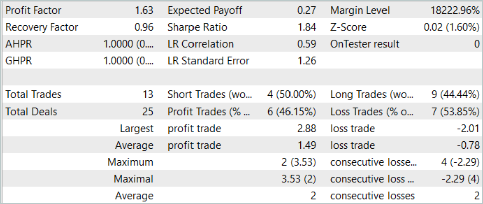
During August 2023, the model executed 13 trades, 6 of which were closed with a profit. The model showed a profit factor of 1.63 during the test period.
Conclusion
In this article, we got acquainted with another method for predicting the upcoming price movement – Multi-future Transformer. One of the key features of this method is the construction of multimodal forecasts for the agent movement with an emphasis on their interaction with each other and with the environmental scene. This allows us to make more accurate forecasts of upcoming movements.
In the practical part, we implemented the proposed approaches using MQL5. We trained and tested the model using real data in the MetaTrader 5 strategy tester. The results obtained confirm the effectiveness of the proposed approaches. We can note the diversity of the obtained forecasts, which is achieved due to the isolation of the forecasts of individual modalities while maintaining the analysis of agent interaction.
References
Programs used in the article
| # | Issued to | Type | Description |
|---|---|---|---|
| 1 | Research.mq5 | Expert Advisor | EA for collecting examples |
| 2 | ResearchRealORL.mq5 | Expert Advisor | EA for collecting examples using the Real-ORL method |
| 3 | Study.mq5 | Expert Advisor | Model training EA |
| 4 | Test.mq5 | Expert Advisor | Model testing EA |
| 5 | Trajectory.mqh | Class library | System state description structure |
| 6 | NeuroNet.mqh | Class library | A library of classes for creating a neural network |
| 7 | NeuroNet.cl | Code Base | OpenCL program code library |
Translated from Russian by MetaQuotes Ltd.
Original article: https://www.mql5.com/ru/articles/14226
 Neural networks made easy (Part 75): Improving the performance of trajectory prediction models
- Free trading apps
- Over 8,000 signals for copying
- Economic news for exploring financial markets
You agree to website policy and terms of use