
Neural networks made easy (Part 75): Improving the performance of trajectory prediction models

Introduction
Forecasting the trajectory of the upcoming price movement probably plays one of the key roles in the process of constructing trading plans for the desired planning horizon. The accuracy of such forecasts is critical. In an attempt to improve the quality of trajectory forecasting, we complicate our trajectory forecasting models.
However, this process also has another side of the coin. More complex models require more computing resources. This means that the costs of both training models and their operation increase. The cost of model training needs to be taken into account. However, as for operating costs, they can be even more critical. Especially when it comes to real-time trading using market orders in a highly volatile market. In such cases, we look at methods to improve the performance of our models. Ideally, such optimization should not affect the quality of future trajectory forecasts.
The trajectory prediction methods we've covered in recent articles were borrowed from the autonomous vehicle driving industry. Researchers in the field are faced with the same problem. Vehicle speeds place increased demands on decision-making time. The use of expensive models for predicting trajectories and making decisions leads not only to an increase in the time spent on decision making, but also to an increase in the cost of the equipment being used as this requires the installation of more expensive hardware. In this context, I suggest considering ideas presented in the article "Efficient Baselines for Motion Prediction in Autonomous Driving". Its authors set the task of building a "lightweight" trajectory forecasting model and highlight the following achievements:
- Identifying a key challenge in the size of movement prediction models with implications for real-time inference and deployment on resource-constrained devices.
- Proposing several effective baselines for vehicle traffic prediction that do not rely explicitly on exhaustive analysis of a high-quality context map, but on prior map information obtained in a simple pre-processing step to serve as a guide to the prediction.
- Using fewer parameters and operations to achieve competitive performance at lower computational cost.
1. Performance improving techniques
Taking into account the balance between the analyzed source data and the complexity of the model, the authors of the method strive to achieve competitive results using powerful deep learning techniques, including attention mechanisms and graph neural networks (GNN). This reduces the number of parameters and operations compared to other methods. In particular, the paper authors use the following as input data for their models:
- past trajectories of agents and their corresponding interactions as the only input to the social base level block
- extension, which adds a simplified representation of the agent's tolerance area as an additional input to the cartographic database.
Thus, the proposed models do not require high quality fully annotated maps or rasterized scene representations to compute physical context.
The authors of the method propose to use a simple but powerful map preprocessing algorithm, where the trajectory of the target agent is initially filtered. Then they compute the feasible area where the target agent can interact, taking into account only the geometric information of the map.
The social baseline uses as input the past trajectories of the most significant obstacles as relative displacements to feed the Encoder module. The social information is then calculated using a Graph Neural Network (GNN). In their paper, the authors of the method use CrystalGraph Convolutional Network (Crystal-GCN), and Multi-Head Self Attention (MHSA) layers to obtain the most significant interactions between agents. After that, in the Decoder module, this latent information is decoded using an autoregressive strategy, in which the output at the i-th step depends on the previous one.
One of the features of the proposed method is the analysis of interaction with agents that have information over the entire time horizon Th = Tobs + Tlen. At the same time, the number of agents that need to be considered in complex traffic scenarios is reduced. Instead of using absolute 2D views from above, the input for the agent i is a series of relative displacements:
![]()
The authors of the method do not limit or fix the number of agents in the sequence. To take into account the relative displacements of all agents, the use one LSTM-block, in which the temporal information of each agent in the sequence is computed.
After encoding the analyzed history of each vehicle in sequence, interactions between agents are computed in order to obtain the most relevant social information. For this purpose, an interaction graph is constructed. The Crystal-GCN layer is used to construct a graph. Then MHSA is applied to improve learning of agent-agent interactions.
Before creating an interaction mechanism, the authors of the method break down temporary information into appropriate scenes. This takes into account that each movement scenario may have a different number of agents. The interaction mechanism is defined as a bidirectional fully connected graph, where the initial node features v0i are represented by latent temporal information for each vehicle hi,out, calculated by the motion history encoder. On the other hand, the edges from the node k to node l are represented by the distance vector ek,l between the corresponding agents at a point in time tobs,len in absolute coordinates:
![]()
Given a graph of interactions (nodes and edges), Crystal-GCN is defined as:
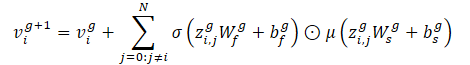
This operator allows us to embed edge features to update node features based on the distance between vehicles. The authors of the method use 2 layers of Crystal-GCN with ReLU and batch normalization as nonlinearities between layers.
σ and μ are the activation functions of sigmoid and softplus, respectively. Besides, zi,j=(vi‖vj‖ei,j) is a concatenation of features of two nodes in the GNN layer and the corresponding edge, N represents the total number of agents in the scene, and W and b are weights and displacements of the corresponding layers.
After passing through the interaction graph, each updated node feature vi contains information about the agent's temporal and social context i. However, depending on the current position and past trajectory, the agent may need to pay attention to specific social information. To model this method, the authors of the method use the multi-headed Self-Attention mechanism with 4 heads, which is applied to the updated node feature matrix V, containing the features of node vi as strings.
Each row of the final social attention matrix SATT (output of the social attention module, after the GNN and MHSA mechanisms) represents an interaction feature for the agent i with surrounding agents, taking into account time information under the hood.
Next, the authors of the method expand the social basic model using minimal information about the map from which they discretize area P of the target agent as a subset of r randomly selected points {p0, p1...pr} around the plausible centerlines (high-level and structured features), taking into account the speed and acceleration of the target agent in the last observation frame. This is a map pre-processing step, so the model never sees the high-resolution map.
Based on the laws of physics, the authors of the method treat the vehicle as a rigid structure without sudden changes in movement between successive time stamps. Accordingly, when describing the task of driving on a road, usually the most important features are in a specific direction (ahead in the direction of movement). This allows the obtaining of a simplified version of the map.
Information about trajectories often contains noise associated with the real-world data collection process. To estimate the dynamic variables of the target agent in the last observation frame tobs,len, the authors of the method propose to first filter past observations of the target agent using a least squares algorithm along each of the axes. They assume that the agent is moving with constant acceleration and they can calculate the dynamic characteristics (velocity and acceleration) of the target agent. Then they compute the vector of velocity and acceleration estimates. Additionally, these vectors are summed as scalars to obtain a smooth estimate, assigning less weight (higher forgetting factor λ) to the first observations. In such a way, most recent observations play a key role in determining the current kinematic state of the agent:
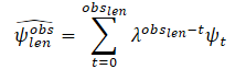
where
obslen is the number of observed frames, ψt is the estimated velocity/acceleration in the frame t, λ ∈ (0, 1) is the forgetting factor.
After calculating the kinematic state, the distance traveled is estimated, assuming a physical model based on acceleration with a constant turning speed at any time t.
These candidate plausible lane trajectories are then processed to be used as plausible physical information. First, they find the closest point to the target agent's last observation that will represent the starting point of a plausible centerline. Then they estimate the distance traveled along the original central lines. They determine the endpoint index p of the centerline m as the point where the accumulated distance (considering the Euclidean distance between each point) is greater than or equal to the pre-computed deviation.
Then they perform cubic interpolation between the start point and end point of the corresponding centerline m to get steps on the planning horizon. Experiments conducted by the authors of the method demonstrate that the best a priori information, taking into account the average and median distance L2 over the entire validation set between the endpoint of the true trajectory of the target agent and the endpoints of the filtered centerlines, is achieved by taking into account the velocity and acceleration in the kinematic state and filtering the input using the method of least squares.
In addition to these high-level and structured centerlines, the authors of the method propose to apply point distortions to all plausible centerlines in accordance with the normal distribution N(0, 0.2). This will discretize the plausible region P as a subset of r randomly selected points {p0, p1...pr} around plausible centerlines. Thus they can get a general idea of the plausible area identified as low-level features. The authors of the method use the normal distribution N as an additional regularization term, instead of using the lane boundaries. This will prevent overfitting in the encoding module, similar to how data augmentation is applied to previous trajectories.
Area and centerline encoders are used to compute latent map information. They process low-level and high-level map features, respectively. Each of these encoders is represented by a multilayer perceptron (MLP). First, they smooth the information along the dimension of the points, alternating the information along the coordinate axes. Then the corresponding MLP (3 layers, with batch normalization, ReLU and DropOut in the first layer) converts interpreted absolute coordinates around the origin into representative latent physical information. The static physical context (output from the region encoder) will serve as a common latent representation for the different modes, while the specific physical context will illustrate specific map information for each mode.
The future trajectory decoder represents the third component of the proposed baseline models. The module consists of an LSTM block that recursively estimates relative movements for future time steps in the same way as the past relative movements were learned in the Motion History Encoder. For the social base case, the model uses the social context computed by the social interaction module, paying attention only to the data of the target agent. The social context alone represents all the traffic in the scenario, representing the input latent vector of the autoregressive LSTM predictor.
From the point of view of the cartographic base case for the mode m, the authors of the method propose to identify the latent traffic context as a concatenation of social context, static physical context and specific physical context, which will serve as an input hidden vector of the LSTM decoder.
Relative to the original data of an LSTM block in the social case, it is represented by encoded past n relative movements of the target agent after spatial embedding, whereas the cartographic baseline adds the encoded distance vector between the target agent's current absolute position and the current centerline, as well as the current scalar timestamp t. In both cases (social and map), the results of the LSTM block are processed using a standard fully connected layer.
After obtaining a relative forecast at a time step t, we shift the initial data of the past observation in such a way as to bring our last calculated relative movement to the end of the vector, removing the first data.
After multimodal predictions are computed, they are concatenated and processed by an MLP residual to gain confidence (the higher the confidence, the more likely the regime is, and the closer to the truth).
The original visualization of the method presented by the paper authors is provided below. Here blue lines represent social information, and red lines display the transfer of information about the card.

2. Implementation using MQL5
We have considered the theoretical aspects of the proposed approach. Now let's implement it using MQL5. As you can see, the authors of the method divided the model into blocks. Each block uses a minimum number of layers. At the same time, simplification of the architecture of individual blocks is accompanied by additional data analysis using a priori information about the analyzed environment. In particular, the map is preprocessed and the trajectories passed are filtered. This allows you to reduce the noise and volume of initial data, without losing the quality of constructing forecast trajectories.
2.1 Creating a CrystalGraph Convolutional Network Layer
In addition, among the proposed approaches we encounter graph neural layers that we have not encountered before. Accordingly, before moving on to building the proposed algorithm, we will create a new layer in our library.
The CrystalGraph Convolutional Network layer proposed by the authors of the method can be represented by the following formula:
Essentially, here we see element-by-element multiplication of the results of the work of 2 fully connected layers. One of them is activated by the sigmoid and represents a trainable binary matrix of the presence of connections between the vertices of the graph. The second layer is activated by the SoftPlus function, which is a soft analogue of ReLU.
To implement CrystalGraph Convolutional Network, we will create a new class CNeuronCGConvOCL inheriting the basic functionality from CNeuronBaseOCL.
class CNeuronCGConvOCL  :  public CNeuronBaseOCL
  {
protected:
   CNeuronBaseOCL    cInputF;
   CNeuronBaseOCL    cInputS;
   CNeuronBaseOCL    cF;
   CNeuronBaseOCL    cS;
   //---
   virtual bool      feedForward(CNeuronBaseOCL *NeuronOCL);
   //---
   virtual bool      updateInputWeights(CNeuronBaseOCL *NeuronOCL);

public:
                     CNeuronCGConvOCL(void) {};
                    ~CNeuronCGConvOCL(void) {};
   //---
   virtual bool      Init(uint numOutputs, uint myIndex, COpenCLMy *open_cl,
                          uint window, uint numNeurons,
                          ENUM_OPTIMIZATION optimization_type,
                          uint batch);
   virtual bool      calcInputGradients(CNeuronBaseOCL *prevLayer);
   //---
   virtual int       Type(void)   const   {  return defNeuronCGConvOCL;   }
   //--- methods for working with files
   virtual bool      Save(int const file_handle);
   virtual bool      Load(int const file_handle);
   virtual CLayerDescription* GetLayerInfo(void);
   virtual bool      WeightsUpdate(CNeuronBaseOCL *source, float tau);
   virtual void      SetOpenCL(COpenCLMy *obj);
  };
Our new class receives a standard set of methods for overriding and basic functionality from the parent class. To implement the graph convolution algorithm, we will create 4 internal fully connected layers:
- 2 for writing the original data and error gradients during the backpropagation pass (cInputF and cInputS)
- 2 to perform the functionality (cF and cS).
We will create all internal objects static, so the constructor and destructor of the class will remain "empty".
In the initialization method of our Init class, we will first call the relevant method of the parent class, which implements all the necessary controls for the data received from the external program and initializes the inherited objects and variables.
bool CNeuronCGConvOCL::Init(uint numOutputs, uint myIndex,
                            COpenCLMy *open_cl, uint window,
                            uint numNeurons,
                            ENUM_OPTIMIZATION optimization_type,
                            uint batch)
  {
   if(!CNeuronBaseOCL::Init(numOutputs, myIndex, open_cl, numNeurons, optimization_type, batch))
      return false;
   activation = None;
After that we sequentially initialize the added internal objects by calling their initialization methods.
   if(!cInputF.Init(numNeurons, 0, OpenCL, window, optimization, batch))
      return false;
   if(!cInputS.Init(numNeurons, 1, OpenCL, window, optimization, batch))
      return false;
   cInputF.SetActivationFunction(None);
   cInputS.SetActivationFunction(None);
//---
   if(!cF.Init(0, 2, OpenCL, numNeurons, optimization, batch))
      return false;
   cF.SetActivationFunction(SIGMOID);
   if(!cS.Init(0, 3, OpenCL, numNeurons, optimization, batch))
      return false;
   cS.SetActivationFunction(LReLU);
//---
   return true;
  }
Please note that for the internal layers of the source data recording, we specified the absence of an activation function. For functional layers, we included the activation functions provided by the algorithm of the created layer. The CNeuronCGConvOCL layer itself does not have an activation function.
After initializing the object, we move on to creating a feed-forward method feedForward. In the parameters, the method receives a pointer to the object of the previous neural layer, the output of which contains the initial data.
bool CNeuronCGConvOCL::feedForward(CNeuronBaseOCL *NeuronOCL)
  {
   if(!NeuronOCL || !NeuronOCL.getOutput() || NeuronOCL.getOutputIndex() < 0)
      return false;
In the method body, we immediately check the relevance of the received pointer.
After successfully passing the block of controls, we need to transfer the source data from the buffer of the previous layer to the buffers of our 2 internal source data layers. Do not forget that we perform all operations with our neural layers on the OpenCL context side. Therefore, we also need to copy data to the memory of the OpenCL context. But we will go a little further and perform "copying" without physically transferring the data. We will simply replace the pointer to the results buffer in the inner layers and pass them a pointer to the results buffer of the previous layer. Here we also indicate the activation function of the previous layer.
   if(cInputF.getOutputIndex() != NeuronOCL.getOutputIndex())
     {
      if(!cInputF.getOutput().BufferSet(NeuronOCL.getOutputIndex()))
         return false;
      cInputF.SetActivationFunction((ENUM_ACTIVATION)NeuronOCL.Activation());
     }
   if(cInputS.getOutputIndex() != NeuronOCL.getOutputIndex())
     {
      if(!cInputS.getOutput().BufferSet(NeuronOCL.getOutputIndex()))
         return false;
      cInputS.SetActivationFunction((ENUM_ACTIVATION)NeuronOCL.Activation());
     }
Thus, when working with internal layers, we get direct access to the results buffer of the previous layer without physically copying the data. We have implemented the task of data transfer with minimal resources. Moreover, we eliminate the creation of two additional buffers in the OpenCL context, thereby optimizing memory usage.
Then we simply call feed-forward methods for the internal functional layers.
   if(!cF.FeedForward(GetPointer(cInputF)))
      return false;
   if(!cS.FeedForward(GetPointer(cInputS)))
      return false;
As a result of these operations, we obtained matrices of context and graph connections. Then we perform their element-wise multiplication. To perform this operation we use the Dropout kernel, which we created for element-by-element multiplication of the original data by a mask. In our case, we have a different background for the same mathematical operation.
Let's pass the necessary parameters and initial data to the kernel.
   uint global_work_offset[1] = {0};
   uint global_work_size[1];
   global_work_size[0] = int(Neurons() + 3) / 4;
   ResetLastError();
   if(!OpenCL.SetArgumentBuffer(def_k_Dropout, def_k_dout_input, cF.getOutputIndex()))
     {
      printf("Error of set parameter kernel %s: %d; line %d", __FUNCTION__,
                                                             GetLastError(), __LINE__);
      return false;
     }
   if(!OpenCL.SetArgumentBuffer(def_k_Dropout, def_k_dout_map, cS.getOutputIndex()))
     {
      printf("Error of set parameter kernel %s: %d; line %d", __FUNCTION__,
                                                             GetLastError(), __LINE__);
      return false;
     }
   if(!OpenCL.SetArgumentBuffer(def_k_Dropout, def_k_dout_out, Output.GetIndex()))
     {
      printf("Error of set parameter kernel %s: %d; line %d", __FUNCTION__,
                                                              GetLastError(), __LINE__);
      return false;
     }
   if(!OpenCL.SetArgument(def_k_Dropout, def_k_dout_dimension, Neurons()))
     {
      printf("Error of set parameter kernel %s: %d; line %d", __FUNCTION__,
                                                              GetLastError(), __LINE__);
      return false;
     }
   if(!OpenCL.Execute(def_k_Dropout, 1, global_work_offset, global_work_size))
     {
      printf("Error of execution kernel %s: %d", __FUNCTION__, GetLastError());
      return false;
     }
//---
   return true;
  }
After that we put it in the execution queue.
The next step is to implement the backpropagation functionality. Here we will start by creating a kernel on the OpenCL side of the program. The point is that the distribution of the error gradient from the previous layer begins with its transfer to the internal layers in accordance with their influence on the final result. To do this, we need to multiply the resulting error gradient by the results of the feed-forward pass of the second functional layer. To avoid calling the element-wise multiplication kernel used above twice, we will create a new kernel in which we will obtain error gradients for both layers in 1 pass.
In the CGConv_HiddenGradient kernel parameters, we will pass pointers to 5 data buffers and the types of activation functions of both layers.
__kernel void CGConv_HiddenGradient(__global float *matrix_g,///<[in] Tensor of gradients at current layer
                                    __global float *matrix_f,///<[in] Previous layer Output tensor
                                    __global float *matrix_s,///<[in] Previous layer Output tensor
                                    __global float *matrix_fg,///<[out] Tensor of gradients at previous layer
                                    __global float *matrix_sg,///<[out] Tensor of gradients at previous layer
                                    int activationf,///< Activation type (#ENUM_ACTIVATION)
                                    int activations///< Activation type (#ENUM_ACTIVATION)
                                   )
  {
   int i = get_global_id(0);
We will launch the kernel in a one-dimensional task space based on the number of neurons in our layers. In the body of the kernel we immediately determine the offset in the data buffers to the element being analyzed based on the thread identifier.
Next, in order to reduce "intensive" operations to access the GPU global memory, we will store the data of the analyzed element in local variables, which are accessed many times faster.
   float grad = matrix_g[i];
   float f = matrix_f[i];
   float s = matrix_s[i];
At this point, we have all the data needed to calculate the error gradients on both layers, and we calculate them.
   float sg = grad * f;
   float fg = grad * s;
But before writing the obtained values into the elements of global data buffers, we need to adjust the found error gradients to the corresponding activation functions.
   switch(activationf)
     {
      case 0:
         f = clamp(f, -1.0f, 1.0f);
         fg = clamp(fg + f, -1.0f, 1.0f) - f;
         fg = fg * max(1 - pow(f, 2), 1.0e-4f);
         break;
      case 1:
         f = clamp(f, 0.0f, 1.0f);
         fg = clamp(fg + f, 0.0f, 1.0f) - f;
         fg = fg * max(f * (1 - f), 1.0e-4f);
         break;
      case 2:
         if(f < 0)
            fg *= 0.01f;
         break;
      default:
         break;
     }
   switch(activations)
     {
      case 0:
         s = clamp(s, -1.0f, 1.0f);
         sg = clamp(sg + s, -1.0f, 1.0f) - s;
         sg = sg * max(1 - pow(s, 2), 1.0e-4f);
         break;
      case 1:
         s = clamp(s, 0.0f, 1.0f);
         sg = clamp(sg + s, 0.0f, 1.0f) - s;
         sg = sg * max(s * (1 - s), 1.0e-4f);
         break;
      case 2:
         if(s < 0)
            sg *= 0.01f;
         break;
      default:
         break;
     }
At the end of the kernel's operation, we save the results of operations into the corresponding elements of global data buffers.
   matrix_fg[i] = fg;
   matrix_sg[i] = sg;
  }
After creating the kernel, we return to working on the methods of our class. The error gradient distribution is implemented in the calcInputGradients method, in the parameters of which we will pass a pointer to the object of the previous layer. In the method body, we immediately check the relevance of the received pointer.
bool CNeuronCGConvOCL::calcInputGradients(CNeuronBaseOCL *prevLayer)
  {
   if(!prevLayer || !prevLayer.getGradient() || prevLayer.getGradientIndex() < 0)
      return false;
Next, we need to call the above-described kernel for distributing the gradient across the internal layers CGConv_HiddenGradient. Here we first define the task space.
   uint global_work_offset[1] = {0};
   uint global_work_size[1];
   global_work_size[0] = Neurons();
Then we pass the necessary parameters to the kernel.
   ResetLastError();
   if(!OpenCL.SetArgumentBuffer(def_k_CGConv_HiddenGradient, def_k_cgc_matrix_f,
                                                             cF.getOutputIndex()))
     {
      printf("Error of set parameter kernel %s: %d; line %d", __FUNCTION__,
                                                         GetLastError(), __LINE__);
      return false;
     }
   if(!OpenCL.SetArgumentBuffer(def_k_CGConv_HiddenGradient, def_k_cgc_matrix_fg,
                                                            cF.getGradientIndex()))
     {
      printf("Error of set parameter kernel %s: %d; line %d", __FUNCTION__,
                                                          GetLastError(), __LINE__);
      return false;
     }
   if(!OpenCL.SetArgumentBuffer(def_k_CGConv_HiddenGradient, def_k_cgc_matrix_s,
                                                               cS.getOutputIndex()))
     {
      printf("Error of set parameter kernel %s: %d; line %d", __FUNCTION__,
                                                           GetLastError(), __LINE__);
      return false;
     }
   if(!OpenCL.SetArgumentBuffer(def_k_CGConv_HiddenGradient, def_k_cgc_matrix_sg,
                                                              cS.getGradientIndex()))
     {
      printf("Error of set parameter kernel %s: %d; line %d", __FUNCTION__,
                                                            GetLastError(), __LINE__);
      return false;
     }
   if(!OpenCL.SetArgumentBuffer(def_k_CGConv_HiddenGradient, def_k_cgc_matrix_g,
                                                                  getGradientIndex()))
     {
      printf("Error of set parameter kernel %s: %d; line %d", __FUNCTION__,
                                                             GetLastError(), __LINE__);
      return false;
     }
   if(!OpenCL.SetArgument(def_k_CGConv_HiddenGradient, def_k_cgc_activationf,
                                                                      cF.Activation()))
     {
      printf("Error of set parameter kernel %s: %d; line %d", __FUNCTION__,
                                                              GetLastError(), __LINE__);
      return false;
     }
   if(!OpenCL.SetArgument(def_k_CGConv_HiddenGradient, def_k_cgc_activations,
                                                                      cS.Activation()))
     {
      printf("Error of set parameter kernel %s: %d; line %d", __FUNCTION__,
                                                              GetLastError(), __LINE__);
      return false;
     }
Put the kernel in the execution queue.
   if(!OpenCL.Execute(def_k_CGConv_HiddenGradient, 1, global_work_offset, global_work_size))
     {
      printf("Error of execution kernel %s: %d", __FUNCTION__, GetLastError());
      return false;
     }
Next we need to propagate the error gradient through the internal fully connected layers. To do this, we call their corresponding methods.
   if(!cInputF.calcHiddenGradients(GetPointer(cF)))
      return false;
   if(!cInputS.calcHiddenGradients(GetPointer(cS)))
      return false;
At this stage we have the results of 2 streams of error gradients on 2 internal layers of the original data. We simply sum them up and transfer the result to the level of the previous layer.
   if(!SumAndNormilize(cF.getOutput(), cS.getOutput(), prevLayer.getOutput(), 1, false))
      return false;
//---
   return true;
  }
Please note that in this case we do not explicitly take into account the activation function of the previous layer anywhere. This is important for the correct transmission of the error gradient. But there is a nuance here. All our classes of neural layers are built in such a way that adjustment to the derivative of the activation function is performed before propagating the gradient to the buffer of the previous layer. For these purposes, during the feed-forward pass, we specified the activation function of the previous layer for our internal layers of the source data. Thus, when the error gradient was propagated through our internal functional layers, we immediately adjusted the error gradient to the derivative of the activation function, which is the same for the gradients of both streams. At the output we sum up the error gradients already adjusted for the derivative of the activation function.
The algorithm of the second backpropagation method (updating the weight matrix updateInputWeights) is quite simple. Here we just call the corresponding methods of the functional internal layers.
bool CNeuronCGConvOCL::updateInputWeights(CNeuronBaseOCL *NeuronOCL)
  {
   if(!cF.UpdateInputWeights(cInputF.AsObject()))
      return false;
   if(!cS.UpdateInputWeights(cInputS.AsObject()))
      return false;
//---
   return true;
  }
The implementation of the remaining methods of our CNeuronCGConvOCL class, in my opinion, is not of particular interest. I used in them the usual algorithms for the corresponding methods, which have already been described many times in this series of articles. You can find them in the attachment. There you will also find the complete code of all programs used when writing the article. Now, let's move on to the implementation of the proposed approaches in building the architecture of models and training them.
2.2 Model architecture
To create architecture of the models, we will use models from the previous articles, keeping the structure of the original data. This is done on purpose. In the ADAPT structure, you can also select an encoder module, which is presented as Feature Encoding. It also includes a block of social attention from successive layers of multi-headed attention. The endpoint prediction block can be compared to the proposed centerlines. The confidence block is similar to predicting trajectory probabilities. This makes working with the new models even more interesting.
bool CreateTrajNetDescriptions(CArrayObj *encoder, CArrayObj *endpoints, CArrayObj *probability)
  {
//---
   CLayerDescription *descr;
//---
   if(!encoder)
     {
      encoder = new CArrayObj();
      if(!encoder)
         return false;
     }
   if(!endpoints)
     {
      endpoints = new CArrayObj();
      if(!endpoints)
         return false;
     }
   if(!probability)
     {
      probability = new CArrayObj();
      if(!probability)
         return false;
     }
Let's start with the encoder model. We feed the model input raw data about the state of the environment.
//--- Encoder
   encoder.Clear();
//--- Input layer
   if(!(descr = new CLayerDescription()))
      return false;
   descr.type = defNeuronBaseOCL;
   int prev_count = descr.count = (HistoryBars * BarDescr);
   descr.activation = None;
   descr.optimization = ADAM;
   if(!encoder.Add(descr))
     {
      delete descr;
      return false;
     }
Raw source data is pre-processed in the batch data normalization unit.
//--- layer 1
   if(!(descr = new CLayerDescription()))
      return false;
   descr.type = defNeuronBatchNormOCL;
   descr.count = prev_count;
   descr.batch = MathMax(1000, GPTBars);
   descr.activation = None;
   descr.optimization = ADAM;
   if(!encoder.Add(descr))
     {
      delete descr;
      return false;
     }
Next, instead of the LSTM block proposed by the authors, I left the Embedding layer with positional coding, since this approach allows us to save and analyze a deeper history.
//--- layer 2
   if(!(descr = new CLayerDescription()))
      return false;
   descr.type = defNeuronEmbeddingOCL;
     {
      int temp[] = {prev_count};
      ArrayCopy(descr.windows, temp);
     }
   prev_count = descr.count = GPTBars;
   int prev_wout = descr.window_out = EmbeddingSize;
   if(!encoder.Add(descr))
     {
      delete descr;
      return false;
     }
//--- layer 3
   if(!(descr = new CLayerDescription()))
      return false;
   descr.type = defNeuronPEOCL;
   descr.count = prev_count;
   descr.window = prev_wout;
   if(!encoder.Add(descr))
     {
      delete descr;
      return false;
     }
I also included a social attention block in the Encoder model. In accordance with the original method, it consists of 2 consecutive graph convolution layers, separated by a layer of batch normalization.
//--- layer 4
   if(!(descr = new CLayerDescription()))
      return false;
   descr.type = defNeuronCGConvOCL;
   descr.count = prev_count * prev_wout;
   descr.window = descr.count;
   if(!encoder.Add(descr))
     {
      delete descr;
      return false;
     }
//--- layer 5
   if(!(descr = new CLayerDescription()))
      return false;
   descr.type = defNeuronBatchNormOCL;
   descr.count = prev_count*prev_wout;
   descr.batch = MathMax(1000, GPTBars);
   descr.activation = None;
   descr.optimization = ADAM;
   if(!encoder.Add(descr))
     {
      delete descr;
      return false;
     }
//--- layer 6
   if(!(descr = new CLayerDescription()))
      return false;
   descr.type = defNeuronCGConvOCL;
   descr.count = prev_count * prev_wout;
   descr.window = descr.count;
   if(!encoder.Add(descr))
     {
      delete descr;
      return false;
     }
The output of the social attention block uses 1 multi-head attention layer.
//--- layer 7
   if(!(descr = new CLayerDescription()))
      return false;
   descr.type = defNeuronMLMHAttentionOCL;
   descr.count = prev_count;
   descr.window = prev_wout;
   descr.step = 4;
   descr.window_out = 16;
   descr.layers = 1;
   descr.optimization = ADAM;
   if(!encoder.Add(descr))
     {
      delete descr;
      return false;
     }
In our case, there is no map of the environment from which we could analytically derive some of the most likely options for the upcoming price movement. Therefore, instead of the central lines, we leave the endpoint prediction block. It will use the results of the social attention block as source data.
//--- Endpoints
   endpoints.Clear();
//--- Input layer
   if(!(descr = new CLayerDescription()))
      return false;
   descr.type = defNeuronBaseOCL;
   prev_count = descr.count = (prev_count * prev_wout);
   descr.activation = None;
   descr.optimization = ADAM;
   if(!endpoints.Add(descr))
     {
      delete descr;
      return false;
     }
But first we need to preprocess the data in a fully connected layer.
//--- layer 1
   if(!(descr = new CLayerDescription()))
      return false;
   descr.type = defNeuronBaseOCL;
   descr.count = LatentCount;
   descr.activation = SIGMOID;
   descr.optimization = ADAM;
   if(!endpoints.Add(descr))
     {
      delete descr;
      return false;
     }
Then we will use the LSTM block, as proposed by the authors of the method for the trajectory decoding block.
//--- layer 2
   if(!(descr = new CLayerDescription()))
      return false;
   descr.type = defNeuronLSTMOCL;
   descr.count = 3 * NForecast;
   descr.activation = None;
   descr.optimization = ADAM;
   if(!endpoints.Add(descr))
     {
      delete descr;
      return false;
     }
At the output of the block, we generate a multi-modal representation of the endpoints for a given number of options.
The model for predicting the probabilities of choosing trajectories remained unchanged. We feed the model the results of the 2 previous models.
//--- Probability
   probability.Clear();
//--- Input layer
   if(!probability.Add(endpoints.At(0)))
      return false;
//--- layer 1
   if(!(descr = new CLayerDescription()))
      return false;
   descr.type = defNeuronConcatenate;
   descr.count = LatentCount;
   descr.window = prev_count;
   descr.step = 3 * NForecast;
   descr.optimization = ADAM;
   descr.activation = SIGMOID;
   if(!probability.Add(descr))
     {
      delete descr;
      return false;
     }
Process them with a block of fully connected layers.
//--- layer 2
   if(!(descr = new CLayerDescription()))
      return false;
   descr.type = defNeuronBaseOCL;
   descr.count = LatentCount;
   descr.activation = LReLU;
   descr.optimization = ADAM;
   if(!probability.Add(descr))
     {
      delete descr;
      return false;
     }
//--- layer 3
   if(!(descr = new CLayerDescription()))
      return false;
   descr.type = defNeuronBaseOCL;
   descr.count = NForecast;
   descr.activation = None;
   descr.optimization = ADAM;
   if(!probability.Add(descr))
     {
      delete descr;
      return false;
     }
Translate the results into the area of probabilities using the SoftMax layer.
//--- layer 4
   if(!(descr = new CLayerDescription()))
      return false;
   descr.type = defNeuronSoftMaxOCL;
   descr.count = NForecast;
   descr.step = 1;
   descr.activation = None;
   descr.optimization = ADAM;
   if(!probability.Add(descr))
     {
      delete descr;
      return false;
     }
//---
   return true;
  }
As in the previous work, we will not attempt to predict the detailed trajectory of price movements. Our main goal is to make a profit in the financial markets. Therefore, we will train an Actor model capable of generating optimal behavior policies based on predicted price movement endpoints.
The model architecture is completely copied from the previous article and is presented in the attachment in the CreateDescriptions method in the file "...\Experts\BaseLines\Trajectory.mqh". Its detailed description is presented in the previous article.
2.3 Model Training
As can be seen from the presented architecture of the models, the sequence of their use in EAs interacting with the environment has remained unchanged. Therefore, in this article we will not dwell on the consideration of algorithms of programs for collecting training data and testing trained models. We go straight to the Model Training Advisor. As in the previous article, all models are trained in one EA “...\Experts\BaseLines\Study.mq5”
In the EA initialization method, we first load a database of examples for training models.
int OnInit()
  {
//---
   ResetLastError();
   if(!LoadTotalBase())
     {
      PrintFormat("Error of load study data: %d", GetLastError());
      return INIT_FAILED;
     }
Then we load pre-trained models and, if necessary, create new ones.
//--- load models
   float temp;
   if(!BLEncoder.Load(FileName + "Enc.nnw", temp, temp, temp, dtStudied, true) ||
      !BLEndpoints.Load(FileName + "Endp.nnw", temp, temp, temp, dtStudied, true) ||
      !BLProbability.Load(FileName + "Prob.nnw", temp, temp, temp, dtStudied, true)
     )
     {
      CArrayObj *encoder = new CArrayObj();
      CArrayObj *endpoint = new CArrayObj();
      CArrayObj *prob = new CArrayObj();
      if(!CreateTrajNetDescriptions(encoder, endpoint, prob))
        {
         delete endpoint;
         delete prob;
         delete encoder;
         return INIT_FAILED;
        }
      if(!BLEncoder.Create(encoder) ||
         !BLEndpoints.Create(endpoint) ||
         !BLProbability.Create(prob))
        {
         delete endpoint;
         delete prob;
         delete encoder;
         return INIT_FAILED;
        }
      delete endpoint;
      delete prob;
      delete encoder;
     }
   if(!StateEncoder.Load(FileName + "StEnc.nnw", temp, temp, temp, dtStudied, true) ||
      !EndpointEncoder.Load(FileName + "EndEnc.nnw", temp, temp, temp, dtStudied, true) ||
      !Actor.Load(FileName + "Act.nnw", temp, temp, temp, dtStudied, true))
     {
      CArrayObj *actor = new CArrayObj();
      CArrayObj *endpoint = new CArrayObj();
      CArrayObj *encoder = new CArrayObj();
      if(!CreateDescriptions(actor, endpoint, encoder))
        {
         delete actor;
         delete endpoint;
         delete encoder;
         return INIT_FAILED;
        }
      if(!Actor.Create(actor) ||
         !StateEncoder.Create(encoder) ||
         !EndpointEncoder.Create(endpoint))
        {
         delete actor;
         delete endpoint;
         delete encoder;
         return INIT_FAILED;
        }
      delete actor;
      delete endpoint;
      delete encoder;
      //---
     }
Then we transfer all models into a single OpenCL context.
   OpenCL = Actor.GetOpenCL();
   StateEncoder.SetOpenCL(OpenCL);
   EndpointEncoder.SetOpenCL(OpenCL);
   BLEncoder.SetOpenCL(OpenCL);
   BLEndpoints.SetOpenCL(OpenCL);
   BLProbability.SetOpenCL(OpenCL);
And control the architecture of the models.
   Actor.getResults(Result);
   if(Result.Total() != NActions)
     {
      PrintFormat("The scope of the actor does not match the actions count (%d <> %d)",
                                                             NActions, Result.Total());
      return INIT_FAILED;
     }
   BLEndpoints.getResults(Result);
   if(Result.Total() != 3 * NForecast)
     {
      PrintFormat("The scope of the Endpoints does not match forecast endpoints (%d <> %d)",

                                                            3 * NForecast, Result.Total());
      return INIT_FAILED;
     }
   BLEncoder.GetLayerOutput(0, Result);
   if(Result.Total() != (HistoryBars * BarDescr))
     {
      PrintFormat("Input size of Encoder doesn't match state description (%d <> %d)",
                                                 Result.Total(), (HistoryBars * BarDescr));
      return INIT_FAILED;
     }
At the end of the method, we create auxiliary data buffers and generate a custom event for the start of model training.
   if(!bGradient.BufferInit(MathMax(AccountDescr, NForecast), 0) ||
      !bGradient.BufferCreate(OpenCL))
     {
      PrintFormat("Error of create buffers: %d", GetLastError());
      return INIT_FAILED;
     }
   if(!EventChartCustom(ChartID(), 1, 0, 0, "Init"))
     {
      PrintFormat("Error of create study event: %d", GetLastError());
      return INIT_FAILED;
     }
//---
   return(INIT_SUCCEEDED);
  }
In the deinitialization method, we save the trained models and clear the memory of dynamic objects.
void OnDeinit(const int reason)
  {
//---
   if(!(reason == REASON_INITFAILED || reason == REASON_RECOMPILE))
     {
      Actor.Save(FileName + "Act.nnw", 0, 0, 0, TimeCurrent(), true);
      StateEncoder.Save(FileName + "StEnc.nnw", 0, 0, 0, TimeCurrent(), true);
      EndpointEncoder.Save(FileName + "EndEnc.nnw", 0, 0, 0, TimeCurrent(), true);
      BLEncoder.Save(FileName + "Enc.nnw", 0, 0, 0, TimeCurrent(), true);
      BLEndpoints.Save(FileName + "Endp.nnw", 0, 0, 0, TimeCurrent(), true);
      BLProbability.Save(FileName + "Prob.nnw", 0, 0, 0, TimeCurrent(), true);
     }
   delete Result;
   delete OpenCL;
  }
The model training process is implemented in the Train method. In the body of the method, we first generate a vector of probabilities for choosing trajectories.
void Train(void)
  {
//---
   vector<float> probability = GetProbTrajectories(Buffer, 0.9);
After that we create local variables.
   vector<float> result, target;
   matrix<float> targets, temp_m;
   bool Stop = false;
//---
   uint ticks = GetTickCount();
Create a system of model training loops.
   for(int iter = 0; (iter < Iterations && !IsStopped() && !Stop); iter ++)
     {
      int tr = SampleTrajectory(probability);
      int batch = GPTBars + 48;
      int state = (int)((MathRand() * MathRand() / MathPow(32767, 2)) *
                        (Buffer[tr].Total - 2 - PrecoderBars - batch));
      if(state <= 0)
        {
         iter--;
         continue;
        }
In the body of the outer loop, we sample the trajectory from the experience replay buffer and the state of the start of learning on it.
Here we will determine the last state of the training package on the selected trajectory and clear the recurrent data buffers.
      BLEncoder.Clear();
      BLEndpoints.Clear();
      int end = MathMin(state + batch, Buffer[tr].Total - PrecoderBars);
In the body of the nested loop, we take one environmental state from the experience replay buffer and run feed-forward passes of the endpoint prediction models and their probabilities.
      for(int i = state; i < end; i++)
        {
         bState.AssignArray(Buffer[tr].States[i].state);
         //--- Trajectory
         if(!BLEncoder.feedForward((CBufferFloat*)GetPointer(bState), 1, false,
                                                           (CBufferFloat*)NULL))
           {
            PrintFormat("%s -> %d", __FUNCTION__, __LINE__);
            Stop = true;
            break;
           }
         if(!BLEndpoints.feedForward((CNet*)GetPointer(BLEncoder), -1, (CBufferFloat*)NULL))
           {
            PrintFormat("%s -> %d", __FUNCTION__, __LINE__);
            Stop = true;
            break;
           }
         if(!BLProbability.feedForward((CNet*)GetPointer(BLEncoder), -1,
                                         (CNet*)GetPointer(BLEndpoints)))
           {
            PrintFormat("%s -> %d", __FUNCTION__, __LINE__);
            Stop = true;
            break;
           }
As you can see, the operations described above are not much different from those in the previous article. But there will be changes. They will specifically concern the transfer of a priori knowledge to the model during the training process. Because by using a priori knowledge about the environment the authors of the method strive to increase the accuracy of forecasts while simplifying the architecture of the models themselves.
In fact, there are several approaches to transferring a priori knowledge to a model. We can pre-process the raw data to compress it and make it more informative. This was proposed by the authors of the method using centerlines.
We can also use a priori knowledge when generating target values in the process of training models. This will help the model pay more attention to the most significant objects in the source data. Of course, it is possible to use both approaches simultaneously.
For the purposes of this article, we will use the second approach. To prepare the target values for the training of the endpoint prediction model, we will first collect upcoming price movement data from the replay buffer.
         targets = matrix<float>::Zeros(PrecoderBars, 3);
         for(int t = 0; t < PrecoderBars; t++)
           {
            target.Assign(Buffer[tr].States[i + 1 + t].state);
            if(target.Size() > BarDescr)
              {
               matrix<float> temp(1, target.Size());
               temp.Row(target, 0);
               temp.Reshape(target.Size() / BarDescr, BarDescr);
               temp.Resize(temp.Rows(), 3);
               target = temp.Row(temp.Rows() - 1);
              }
            targets.Row(target, t);
           }
         target = targets.Col(0).CumSum();
         targets.Col(target, 0);
         targets.Col(target + targets.Col(1), 1);
         targets.Col(target + targets.Col(2), 2);
As an example of a priori knowledge, we will use the signals of the MACD indicator. Our main line data is stored in element 7 of the array describing the state of the environment. The value of the signal line is in element 8 of the same array. If the signal line is above the main line, then we consider the current trend to be bullish. Otherwise, bearish.
int direct = (Buffer[tr].States[i].state[8] >= Buffer[tr].States[i].state[7] ? 1 : -1);
I agree that this approach is quite simplified and we could use more signals and indicators to identify trends. But precisely this simplicity will provide a clear example of implementation within the framework of the article and will allow us to evaluate the impact of the approach. I suggest you use more comprehensive approaches in your projects to obtain optimal results.
After determining the direction of the trend, we determine the extremum in this direction. We also limit the matrix of the upcoming price movement to the found extremum.
         ulong extr=(direct>0 ? target.ArgMax() : target.ArgMin());
         if(extr==0)
           {
            direct=-direct;
            extr=(direct>0 ? target.ArgMax() : target.ArgMin());
           }
         targets.Resize(extr+1, 3);
It should be noted here that the MACD signal lags behind trend changes. Therefore, if, when determining the extremum, we find it in the first row of the matrix, we change the direction of the trend to the opposite and redefine the extremum.
By using trends determined using a priori knowledge of the environment, we somewhat reduce the stochasticity of target values that was previously observed when using the direction of the first upcoming candle. In general, this should help our model more correctly determine trends and future directions of price movement.
From the truncated matrix of the upcoming price movement, we determine the target values by the extremum of the upcoming price movement.
         if(direct >= 0)
           {
            target = targets.Max(AXIS_HORZ);
            target[2] = targets.Col(2).Min();
           }
         else
           {
            target = targets.Min(AXIS_HORZ);
            target[1] = targets.Col(1).Max();
           }
As before, we determine the most accurate model forecast from the entire multi-modal endpoint space and, in a backpropagation run, adjust only the selected prediction.
         BLEndpoints.getResults(result);
         targets.Reshape(1, result.Size());
         targets.Row(result, 0);
         targets.Reshape(NForecast, 3);
         temp_m = targets;
         for(int i = 0; i < 3; i++)
            temp_m.Col(temp_m.Col(i) - target[i], i);
         temp_m = MathPow(temp_m, 2.0f);
         ulong pos = temp_m.Sum(AXIS_VERT).ArgMin();
         targets.Row(target, pos);
         Result.AssignArray(targets);
The target values prepared in this way allow us to update the parameters of the endpoint prediction model and the initial environmental state Encoder.
         if(!BLEndpoints.backProp(Result, (CBufferFloat*)NULL))
           {
            PrintFormat("%s -> %d", __FUNCTION__, __LINE__);
            Stop = true;
            break;
           }
         if(!BLEncoder.backPropGradient((CBufferFloat*)NULL))
           {
            PrintFormat("%s -> %d", __FUNCTION__, __LINE__);
            Stop = true;
            break;
           }
Here we adjust the probability forecasting models. But we don't transmit the error gradient of this model to the endpoint prediction model or the Encoder.
         bProbs.AssignArray(vector<float>::Zeros(NForecast));
         bProbs.Update((int)pos, 1);
         bProbs.BufferWrite();
         if(!BLProbability.backProp(GetPointer(bProbs), GetPointer(BLEndpoints)))
           {
            PrintFormat("%s -> %d", __FUNCTION__, __LINE__);
            Stop = true;
            break;
           }
The next step is to train the Actor policy. Here we first prepare information about the account status and open positions.
         //--- Policy
         float PrevBalance = Buffer[tr].States[MathMax(i - 1, 0)].account[0];
         float PrevEquity = Buffer[tr].States[MathMax(i - 1, 0)].account[1];
         bAccount.Clear();
         bAccount.Add((Buffer[tr].States[i].account[0] - PrevBalance) / PrevBalance);
         bAccount.Add(Buffer[tr].States[i].account[1] / PrevBalance);
         bAccount.Add((Buffer[tr].States[i].account[1] - PrevEquity) / PrevEquity);
         bAccount.Add(Buffer[tr].States[i].account[2]);
         bAccount.Add(Buffer[tr].States[i].account[3]);
         bAccount.Add(Buffer[tr].States[i].account[4] / PrevBalance);
         bAccount.Add(Buffer[tr].States[i].account[5] / PrevBalance);
         bAccount.Add(Buffer[tr].States[i].account[6] / PrevBalance);
         double time = (double)Buffer[tr].States[i].account[7];
         double x = time / (double)(D'2024.01.01' - D'2023.01.01');
         bAccount.Add((float)MathSin(x != 0 ? 2.0 * M_PI * x : 0));
         x = time / (double)PeriodSeconds(PERIOD_MN1);
         bAccount.Add((float)MathCos(x != 0 ? 2.0 * M_PI * x : 0));
         x = time / (double)PeriodSeconds(PERIOD_W1);
         bAccount.Add((float)MathSin(x != 0 ? 2.0 * M_PI * x : 0));
         x = time / (double)PeriodSeconds(PERIOD_D1);
         bAccount.Add((float)MathSin(x != 0 ? 2.0 * M_PI * x : 0));
         if(bAccount.GetIndex() >= 0)
            bAccount.BufferWrite();
Then we create Embeddings of states and predicted endpoints.
         //--- State embedding
         if(!StateEncoder.feedForward((CNet *)GetPointer(BLEncoder), -1,
                                       (CBufferFloat*)GetPointer(bAccount)))
           {
            PrintFormat("%s -> %d", __FUNCTION__, __LINE__);
            Stop = true;
            break;
           }
         //--- Endpoint embedding
         if(!EndpointEncoder.feedForward((CNet *)GetPointer(BLEndpoints), -1,
                                           (CNet*)GetPointer(BLProbability)))
           {
            PrintFormat("%s -> %d", __FUNCTION__, __LINE__);
            Stop = true;
            break;
           }
Note that, unlike previous work, we use the results of the feed-forward pass above the trained models to generate the embedding of the predictive endpoints, rather than the target values. This will allow us to tailor the Actor's performance to the results of the endpoint prediction model.
After preparing the embeddings, we perform a feed-forward pass through the Actor model.
         //--- Actor
         if(!Actor.feedForward((CNet *)GetPointer(StateEncoder), -1,
                               (CNet*)GetPointer(EndpointEncoder)))
           {
            PrintFormat("%s -> %d", __FUNCTION__, __LINE__);
            Stop = true;
            break;
           }
Successful execution of the feed-forward pass is followed by a backward pass that updates the model parameters. Here, when preparing target values for training the actor model, we will also add some a priori knowledge. In particular, before opening a trade in one direction or another, we will check the values of the RSI and CCI indicators, which are stored in the 4th and 5th elements of the environmental state description array, respectively.
         if(direct > 0)
           {
            if(Buffer[tr].States[i].state[4] > 30 &&
               Buffer[tr].States[i].state[5] > -100
              )
              {
               float tp = float(target[1] / _Point / MaxTP);
               result[1] = tp;
               int sl = int(MathMax(MathMax(target[1] / 3, -target[2]) / _Point, MaxSL / 10));
               result[2] = float(sl) / MaxSL;
               result[0] = float(MathMax(risk / (value * sl), 0.01)) + FLT_EPSILON;
              }
           }
         else
           {
            if(Buffer[tr].States[i].state[4] < 70 &&
               Buffer[tr].States[i].state[5] < 100
              )
              {
               float tp = float((-target[2]) / _Point / MaxTP);
               result[4] = tp;
               int sl = int(MathMax(MathMax((-target[2]) / 3, target[1]) / _Point, MaxSL / 10));
               result[5] = float(sl) / MaxSL;
               result[3] = float(MathMax(risk / (value * sl), 0.01)) + FLT_EPSILON;
              }
           }
Please note that in this case we are not explicitly checking the MACD indicator signals, since they have already been taken into account when determining the direction of the upcoming movement direct.
With these prepared target values, we can execute a backpropagation pass through the composite Actor model.
         Result.AssignArray(result);
         if(!Actor.backProp(Result, (CNet *)GetPointer(EndpointEncoder)) ||
            !StateEncoder.backPropGradient(GetPointer(bAccount),
                                           (CBufferFloat *)GetPointer(bGradient)) ||
            !EndpointEncoder.backPropGradient((CNet*)GetPointer(BLProbability))
           )
           {
            PrintFormat("%s -> %d", __FUNCTION__, __LINE__);
            Stop = true;
            break;
           }
We use the Actor error gradient to update the Encoder parameters, but we do not update the endpoint prediction model.
         if(!BLEncoder.backPropGradient((CBufferFloat*)NULL))
           {
            PrintFormat("%s -> %d", __FUNCTION__, __LINE__);
            Stop = true;
            break;
           }
At the end of the operations within the loop system, we just need to inform the user about the progress of the training process.
         if(GetTickCount() - ticks > 500)
           {
            double percent = (double(i - state) / ((end - state)) + iter) * 100.0 /
                                                                       (Iterations);
            string str = StringFormat("%-14s %6.2f%% -> Error %15.8f\n", "Actor",
                                            percent, Actor.getRecentAverageError());
            str += StringFormat("%-14s %6.2f%% -> Error %15.8f\n", "Endpoints",
                                      percent, BLEndpoints.getRecentAverageError());
            str += StringFormat("%-14s %6.2f%% -> Error %15.8f\n", "Probability",
                                    percent, BLProbability.getRecentAverageError());
            Comment(str);
            ticks = GetTickCount();
           }
        }
     }
After completing the model training process, we clear the comments field on the chart. Output the model training results to the log and initiate the EA termination process.
   Comment("");
//---
   PrintFormat("%s -> %d -> %-15s %10.7f", __FUNCTION__, __LINE__,

                                       "Actor", Actor.getRecentAverageError());
   PrintFormat("%s -> %d -> %-15s %10.7f", __FUNCTION__, __LINE__,
                             "Endpoints", BLEndpoints.getRecentAverageError());
   PrintFormat("%s -> %d -> %-15s %10.7f", __FUNCTION__, __LINE__,
                         "Probability", BLProbability.getRecentAverageError());
   ExpertRemove();
//---
  }
This concludes our consideration of algorithms for implementing the proposed basic approaches to optimizing trajectory prediction models. And you can find the complete code of all programs used herein in the attachment.
3. Testing
We have implemented basic approaches to optimizing trajectory forecasting models using MQL5. In particular, we have created a graph convolution layer and applied approaches to use a priori knowledge about the environment when setting goals during model training. This has reduced the number of layers in the models, which should potentially reduce the complexity of the models and increase the speed of their operation. We assessed the impact of the proposed approaches in the process of training and testing the trained models on real data in the MetaTrader 5 strategy tester.
As before, training and testing of models is carried out on the first 7 months of 2023 of EURUSD H1.
When building the architecture of models, we already mentioned the preserving of the source data structure. This allowed us to use in training the experience replay buffer collected in previous articles. We simply rename the previously collected data file to BaseLines.bd. If you want to create a new training dataset, you can use any of the previously discussed methods using environmental interaction EAs.
The process of generation of target values during the model training process allowed us to use the training dataset until we obtain optimal results without the need to update and supplement it.
However, the training results turned out to be not as promising as expected. When testing trained models, we increased the testing period from 1 to 3 months.


Well, we managed to obtain a model capable of generating profit on both the training and test samples. Moreover, the resulting model demonstrated good stability with a profit factor of 1.4. After training on historical data for 7 months, the model is able to generate profits for at least 3 months. This may indicate that the model was able to identify fairly stable predictors.
However, the model was quite poor in terms of the number of trades. 11 trades completed in 3 months is very little. This is not the result we wanted to achieve.
Conclusion
In this article, we examined basic approaches to optimizing the performance of trajectory prediction models. The implementation of the proposed approaches makes it possible to train models capable of identifying truly significant predictors in the source data. This allows stable operation for a fairly long period of time after training.
However, our results indicate strong conservatism in the decisions made by the models. This is reflected in a very small number of deals made. So, this is the direction in which we have to continue research.
References
Programs used in the article
| # | Issued to | Type | Description |
|---|---|---|---|
| 1 | Research.mq5 | Expert Advisor | Example collection EA |
| 2 | ResearchRealORL.mq5 | Expert Advisor | EA for collecting examples using the Real-ORL method |
| 3 | Study.mq5 | Expert Advisor | Model training EA |
| 4 | Test.mq5 | Expert Advisor | Model testing EA |
| 5 | Trajectory.mqh | Class library | System state description structure |
| 6 | NeuroNet.mqh | Class library | A library of classes for creating a neural network |
| 7 | NeuroNet.cl | Code Base | OpenCL program code library |
Translated from Russian by MetaQuotes Ltd.
Original article: https://www.mql5.com/ru/articles/14187
 Neural networks made easy (Part 76): Exploring diverse interaction patterns with Multi-future Transformer
- Free trading apps
- Over 8,000 signals for copying
- Economic news for exploring financial markets
You agree to website policy and terms of use